Table of Contents
TL;DR
-
Using machine learning models on multiple datasets, an attempt was made to improve upon the UN’s fertility rate forecasting methods, achieving better short-term accuracy.
-
Adding education gender gaps, child mortality rates, and data from pre-1950 improved model performance, while factors like population density and geographic location were less useful.
-
The best models reduced forecast error by ~40% compared to UN projections when tested on high-quality data from developed nations, but still struggled with extreme cases like South Korea.
-
Long-term forecasting to 2100 remains challenging, with potential improvements possible through country-specific modeling and better handling of historically low fertility rates.
Introduction
A few months ago, I attempted to take on the UN’s population division. Mostly because nobody other than large multi-national NGOs seemed interested.
It was moderately harder than I thought it would be, but in the end - as someone in your life has probably told you - it was about the journey, not the destination. I ended up in a different place coming out of this analysis than I though I’d be, but I think there’s sufficient information to impart with.
Some Overview
Biannually the UN publishes their “World Population Prospects” in which they comprehensively reassess past, present and future populations by re-estimating fertility, mortality, and international migration for each age group by sex. This is broadly known as the “cohort-component method”. After this re-evaluation, they project future populations forward to 2100. However, lately, these projections have become controversial, as they’ve been shown to consistently, almost comically, fail. Here’s a showcase of the UN’s best:
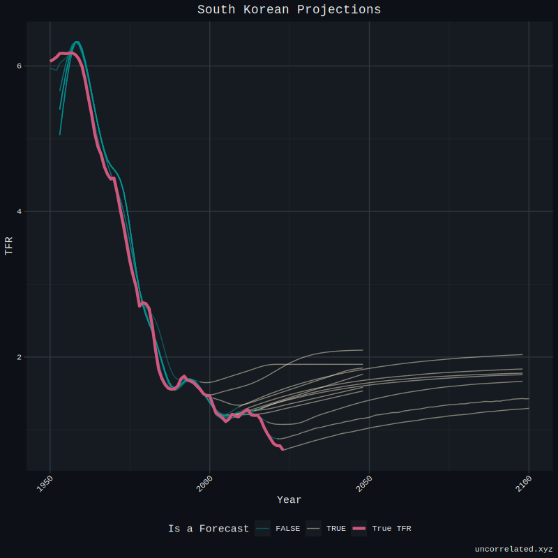
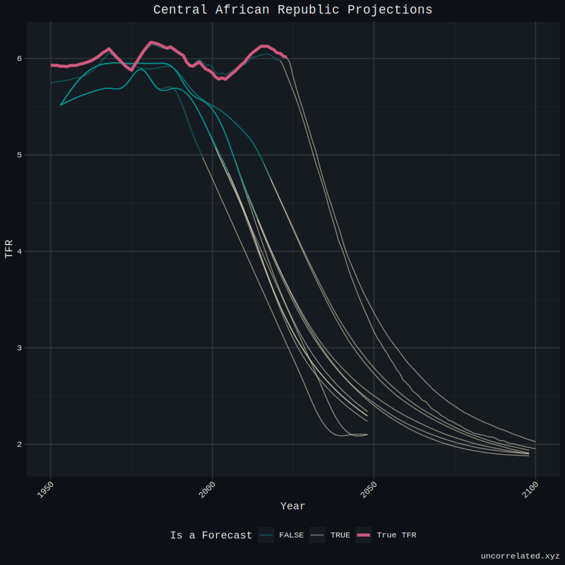
This post isn’t about the technical details of the UN’s forecasting method, or how they estimate present and past fertility: the UN’s methodology and Spoonberg, 2020 offer a sufficient overview.
Instead, our approach was more direct: develop alternative fertility projections and compare against the UN’s.
To do this, we will use machine learning. And following machine learning, we must use its methods. Very broadly speaking, machine learning follows a formula. You split your data into a training, validation and test set. The training set is - as the name suggests - for training any sort of model you can think of. The validation set is to validate any and all of the models that were created in training, however, the test set is for evaluating the final model, yielded from the best in the validation set.
At the time I did this analysis I decided NOT to make a test set. In retrospect, this was regretted. I will explain more in the conclusion.
With that outline, it is prudent that we care for the data. Which leads us to our first section; how I curated it for ML.
Our Data, Their Data
Something you may have noticed in our first figure is that the historical TFR fluctuated from population prospect to population prospect. That’s correct! The reason for this is obvious if we highlight the UN’s methodology.
At the global level, population data from censuses or registers referring to 2019 or later were available for 114 countries or areas, representing 48 per cent of the 237 countries or areas … (54 per cent of the world population).
For 43 countries or areas, the most recent available population count was from the period 2014-2018, and for another 57 locations from the period 2009-2013.
For the remaining 23 countries or areas, the most recent available census data were from before 2009, that is more than 15 years ago. These 23 countries (with date of last census) were Lebanon (1932), Afghanistan (1979), Democratic Republic of the Congo (1984), Eritrea (1984), Somalia (1987), Uzbekistan (1989), Iraq (1997), Ukraine (2001), Haiti (2003), Syrian Arab Republic (2004), Yemen (2004), Cameroon (2005), Nicaragua (2005), United Arab Emirates (2005), Libya (2006), Nigeria (2006), El Salvador (2007), Ethiopia (2007), Algeria (2008), Burundi (2008), Dem. People’s Republic of Korea (2008), South Sudan (2008) and Sudan (2008).
So for roughly half the world’s population, we don’t have recent population registers or censuses conducted in the past 5 years!
This lack of data can cause massive discrepancies between estimates and reality, as is seen in Spoonberg, 2020.
A recent example is the case of Myanmar where, in the absence of a population census since 1983, official estimates put the population of the country to 62 million in 2012. This figure is about 10 million lower than the population enumerated in the 2014 population census. The official population estimates were based on outdated population projections that did not account properly for the changes in fertility and international migration (Spoorenberg, 2013).
The UN acknowledges this, and thus, many estimates up until Jan 1st 2024 are not reflections of carefully curated government data reports but simply UN projections. Here they say this:
In the 2024 revision, the figures from 1950 up to 2023 are treated as estimates, and thus the projections for each country or area begin on 1 January 2024 and extend until 2100. Because population data are not necessarily available for that date, the 2024 estimate is derived from the most recent population data available for each country, obtained usually from a population census or a population register, projected to 2024 using all available data on fertility, mortality and international migration trends between the reference date of the population data available and 1 January 2024.
This is critical for our forecasting task, because, in effect, it means if we train on the data uploaded by the UN WPP 2024, we’re not just forecasting the real TFR but the behavior of the UN’s model. If we don’t adjust for this, our validation metrics will seem much better than they are in reality because it’s far easier to predict the UN’s model than it is to predict the future.
Luckily for us, the UN provides distinctions between interpolation and projection for their estimates. We can see this here with the fertility of syria.
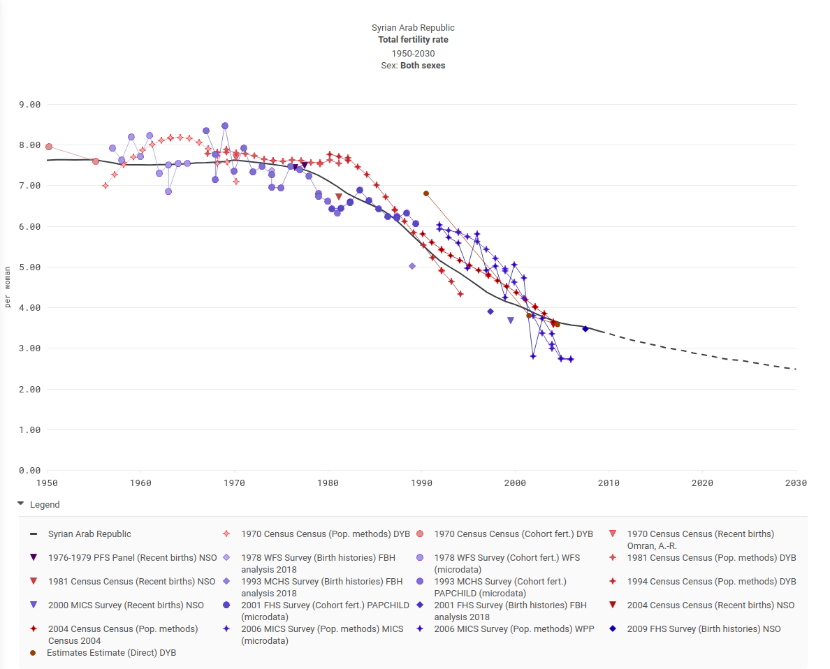
So, for the dataset from which we’ll be training our machine learning models we will exclude all “projection” years.
Finally, for the most recent years that aren’t projections, anons like @birthgauge and others have reported fertility that diverges from UN estimates significantly. After excluding ‘projected’ data from the UN’s WPP, the gap between these two sourced collapsed significantly. As a result, we will not be taking birthgauge’s values over the UN’s, the differences after this adjustment are firstly, tiny, and secondly, from what’s been seen, the UN is more involved in adjusting birth rates for over or under representation, often drawing on multiple sources for poorer countries. To my knowledge birthgauge does not do this. He might be he certainly doesn’t publish his method. So we’d rather go with the method that’s more transparent.
Although it might seem somewhat hypocritical, the quality of much older historical TFR estimates is not as important. If we include data dating back to 1800, and the inclusion of that data improves the model’s ability to predict on unseen, future data, then there’s no reason not to include it despite issues with accuracy. This obviously doesn’t hold for validation data because that’s the yardstick for our model.
The UN’s machine learning approach is univariate. This is just to say that their model doesn’t also consider mortality, GDP, education, etc. It uses TFR to predict TFR, simple as.
For us, we will consider an expanded multivariate dataset, that way, we will give our model the best chance to learn the contours and dynamics of fertility as it relates to the world (variables) around it. We will explain the rationality behind the inclusion or exclusion of each: National IQ, male female education ratio, population weighted density, child mortality rate, general trends, GDP.
Total Fertility Rate
The first source we’re relying on is TFR from GapMinder. They provide fertility estimates dating back to 1800 for most countries. Of course, most estimates for most countries simply plateau into guesstimates the further one goes back. This is useless data that is likely toxic to our machine learning models – we don’t want it to learn overly noisy features but to focus on real data. As a result, any TFR estimate that “basically” doesn’t change for 70 consecutive years is removed.
Feature Engineering
It’s common to provide data that spoonfeeds the trends for machine learning models to pick up. For example, let’s say we wanted to predict the stockmarket. Instead of just giving the everyday closing price, we might also provide the model with how many consecutive days there’s been a decrease or increase, the moving average of the price, the month of the year, the difference from the previous day, etc. This is known as feature engineering. It spoonfeeds the model the best features to learn from, giving crutches to learn. We are doing the same to our model, we will provide the exponential moving average of fertility. Importantly however, these features MUST NOT include future years in its calculation. Many, many time series analysis tools do this. For example, I was recommended the Hodrick-Prescott filters from a book I read on time series forecasting. This caused massive data leakage in my models instantly. I emailed the author as to why they suggested this, they never got back.
Child Mortality Rate
Once again, we turn to GapMinder, which has child mortality rates by country dating back to 1800. Since GapMinder already provides the data, there’s nothing to lose by adding it.
National IQ
NIQ, might be a decent at forecasting fertility, but it comes with caveats.
-
NIQ is better at predicting fertility than fertility, up to a point.
A post by sebastian jensen showed that NIQ has greater validity at predicting present day TFR than TFR in the 50s.
I was curious to see the threshold for when NIQ ceases to be superior at predicting present TFR than historical TFR, so I ran an OLS regression for every year, predicting 2020. So, 2020 ~ 1951 + niq, 2020 ~ 1952 + niq, 2020 ~ 1952 + niq, etc. These are the respective p-values for each.
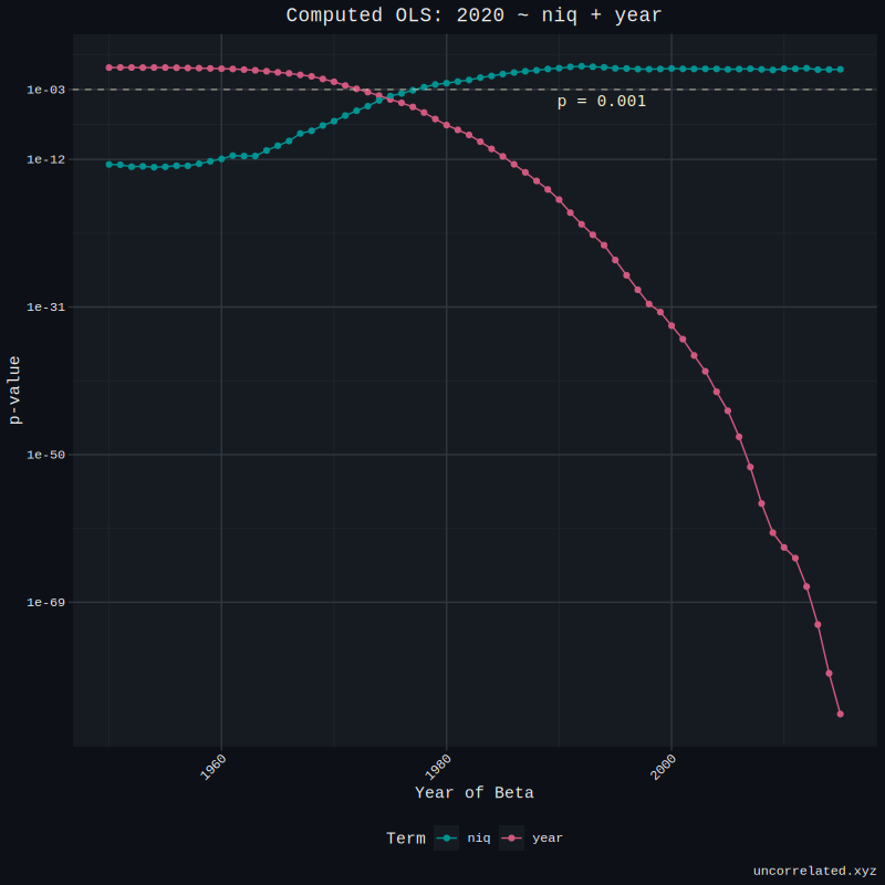
As you can see, TFR seems to overtake IQ in predicting 2020’s fertility around about the mid 70s. This means that IQ is about just as good at predicting present fertility as historic fertility about 45 years ago.
We must consider that the NIQ’s advantage in historical years may be due to a data leakage. Put simply, NIQ is based on measurements basically made for the present day. This means that if we use it to predict future TFR, we’re including information about the future in past models, which is cheating since it would be impossible to literally measure what NIQ would be in 2020 in the year 1950. But this leads us to our second point.
-
NIQ is mostly constant.
This is more of an assumption inherent to NIQ. NIQ does obviously change, especially over the timescales we’re interested in - which is decades. However, it should be mostly constant, not changing more than a few points at most. This limits the extent to which leakage can theoretically take place. Anyway, when we go through hyperparameter tuning, we will find out whether this is true.
-
NIQ is one of if not the best predictor of current and future economic performance. Francis, Kirkegaard 2022. Personally I don’t think this paper is comprehensive enough (although the findings would likely replicate). Despite this, it makes intuitive sense. Ghana and Korea achieved independence at roughly the same time, the latter went through multiple extremely devastating conflicts, North Korea went through communism, yet the North still finds itself winning maths Olympiads and making nuclear weapons, with the South - relative to Ghana - prospering immensely. Economics affects education, development, access to contraceptives, etc. IQ isn’t terribly predictive of fertility within a country, but between it it is significant because its effects compound to alter its society. You can see this in the next point.
Simple thought experiment for why IQ matters more than you might think: It multiplies.
Lets say that, in an all-black country, the median car mechanic makes 3x more mistakes than the median car mechanic in an all white country.
Not good, but functional. You can get by fine with 3x as many car mechanic errors.
But you also have black drivers. Lets say black drivers are 3x as likely, over a given time frame for any given make and model, to mess up their car. Okay, now you have 3x as many cars needing fixing, so your mechanic errors and return trips to re-fix the problem is 9x.
We’ll pass on the idea of all-black countries making their own cars.
Now, add to this, in all black-countries, you tend to get lower-end, older cars which start to have problems. Lets say these are 3x more likely to have problems, for a given level of maintenance.
So where are we? The cars are inherently 3x more likely to have some issue, the drivers are 3x more likely to mess something up, and the mechanics are 3x more likely to botch the repair. So 27x as many botched car repair jobs.
Everything is like this, to some degree. There’s no one point that you can look at and go “aha, this is where they’re messing up!”, because it multiplies on itself.
Combining these four points, it’s evident that NIQ has and will continue to be a predictor of past, present and future prosperity, growth, economic and hence social and demographic change. Who knows, maybe it won’t actually improve the predictive validity of our forecast, or only do so mildly. I leave it up to the data and the machine learning.
Lived Population Density
Some folks have reviewed some of the population density question, Lyman Stone, Noal Carl and Bo Winegard, Sebastian Jensen, Kirkegaard.
Moreover, their collective findings could be summarized like this:
- Effect sizes are small.
- Little or no correlation between countries.
- Small correlation between individuals or small administrative units (counties, instead of states or countries).
Personally, I downloaded the HYDE 3.3 geospatial population dataset. Here’s a visualization of Brazil.
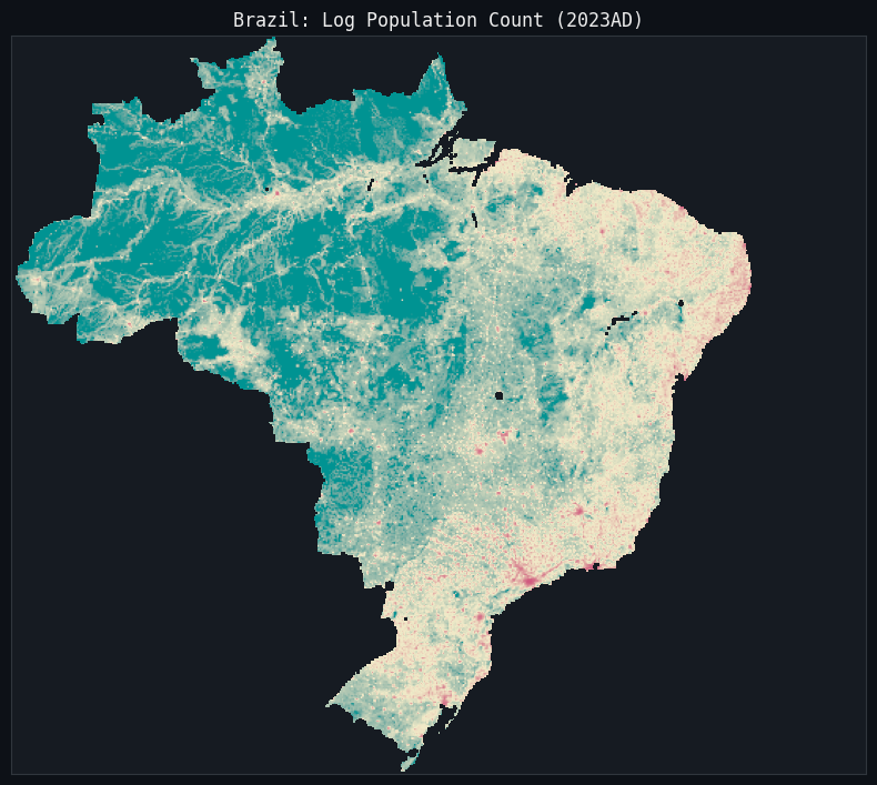
I was interested in computing the ’lived population density’ by country, then seeing if it can predict fertility between countries.
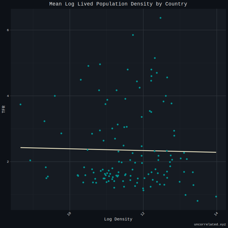
Needless to say, the results were not exciting. This did corroborate what the others found - Noah and Bo. In my opinion I think the folks that choose to live in high-density dwellings are selected, rather than there being a causal mechanism. So Given the mixed results on an international scale, I decided to exclude population density from my analysis.
Male / Female Education Ratio
A year ago, Arctotherium published an article. His underpinning observation is that many correlates of fertility between countries today and across time reversed during the baby boom. Most significantly, he highlights the education gap between men and women as one of the main causal drivers that elevated fertility during this period.
A means to test this hypothesis is to add education gaps to our models. Should they enhance their ability to predict unseen data, it should follow that there is perhaps a truth to it.
So, we need to find a source of education data that can cover most countries for which we already have fertility data, and that covers a sufficient period of time to 1800.
The first dataset I found was a compilation of sources from Our World In Data. This data was accessed before its latest update on November. For many countries, estimates for enrollment in primary, secondary and tertiary education is provided.
However, this data has “more holes than swiss cheese” as they say. The first step to ameliorate this was to do linear interpolation between datapoints.
Despite this, many countries still had vast swaths of missing years, particularly well into the past. If a country had near zero enrollment rates for any category, it was assumed this was so the case into the deep past, and so the first observation in many cases was carried backwards.
Lastly, some countries still had extremely poor records, for example, Somalia had data for only a handful of years in the 1970s and 1980s. That’s far from having data continuously from 1800 to the present day. Missing data like this is so severe that we need to turn to machine learning. For our purposes, that will be SAITS or “Self-Attention-based Imputation for Time Series.” Imputation is quite common in the timeseries literature, with SoTA (state of the art) ML techniques being continuously developed.
But that still likely won’t be enough.
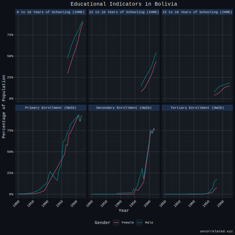
Luckily for Somalia and others, we have the IHME’s Global Educational Attainment Distributions which provides educational attainment estimates for again most countries between 1970-2030. We can add this to SAITS, and the model should be capable of leveraging the relationship that exists between IHME’s and OWID’s dataset to impute the missing data not present in OWID. We can see Bolivia as an example where this is most useful. As seen below, tertiary data does not exist in OWID’s, but does for IHME.
I didn’t spend any rigorous time validating SAITS. Too much time could be spent just improving impute accuracy of just this metric. Like with the fertility data dating back to the 1800s, we’re simply looking for data that is ‘good enough’ not a perfect representation of educational attainment, and should education gaps genuinely aid in forecasting fertility, time should be spent improving impute accuracy then. So what was accomplished here should be sufficient for now.
After completing the imputation of the data, we need to use it to compute gender gaps in education. A ratio was settled on; male education / female education. However, education is split into three categories in this data, primary, secondary and tertiary.
A formula was settled on:
Step 1: Calculate the weighted sum for males and females. $$M_{weighted} = 3M_t + 2M_s + M_p + 0.0001$$ $$F_{weighted} = 3F_t + 2F_s + F_p + 0.0001$$ This gives triple weight to tertiary education, double to secondary, and single to primary education.
Step 2: Calculate the initial ratio $$ratio_{initial} = \frac{M_{weighted}}{F_{weighted}}$$ This divides the male weighted sum by the female weighted sum. The tiny 0.0001 was added to prevent ludicrous values where female education does not exist.
Step 3: Bound the result to a maximum value of 5, and a minimum value of 0.2 $$ratio_{max} = \min(ratio_{initial}, 5)$$ $$ratio_{bounded} = \max(ratio_{max}, 0.2)$$ If the ratio is larger than 5, set it to 5, If the ratio is smaller than 0.2, set it to 0.2.
Step 4: Take the natural logarithm $$ratio_{final} = \log(ratio_{bounded})$$ This transforms the ratio to make it more symmetrical around zero. It also again helps to deal with absurd values.
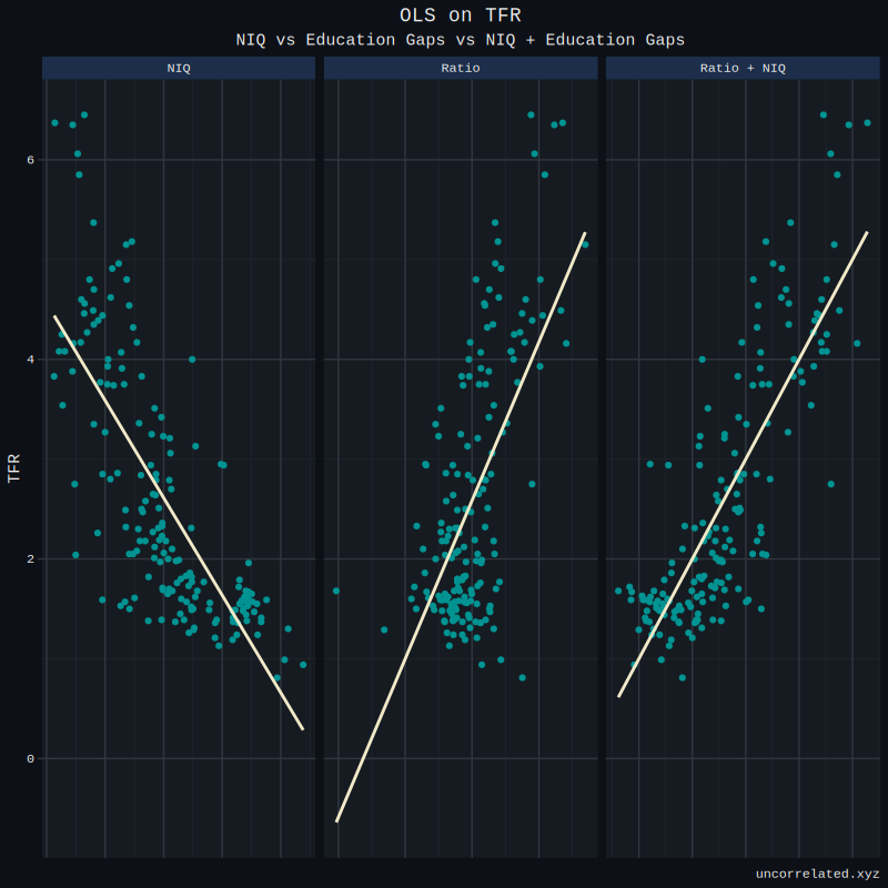
Finally, does this ratio - controlling for NIQ - predict TFR in any single year? We can test this with a simple OLS model. We’ll just use international data for the year 2020. Before making the OLS model, Ratio and NIQ were standardized. Very clearly, ratio and niq appear to be extremely significant.
  term        estimate std.error statistic  p.value
  <chr>          <dbl>     <dbl>     <dbl>    <dbl>
1 (Intercept)    2.60     0.0565     46.1  6.01e-98
2 ratio          0.462    0.0618      7.48 3.77e-12
3 niq           -0.766    0.0633    -12.1  1.01e-24
We can visualize this, and observe with our own eyes that yes, in fact, adding the gap in educational attainment between the sexes improve predictive ability.
Okay, this works for the year 2020, however, does it work for all years between countries? Below, we can see that the beta for ratio, adjusting for NIQ, ceases to be significant just before the 70s, and the ability or NIQ and ratio to jointly predict TFR deteriorates continuously.
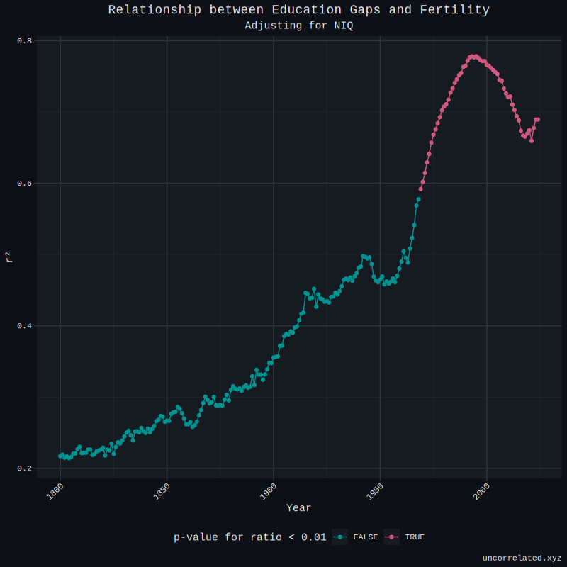
What predicts fertility across time likely changes, in a addition to the fact that the measurement of historical data - TFR, education gaps and NIQ - all declines in accuracy. Resulting in increased error, noisier correlations and weaker betas. However, I think the former is more likely true, that educational gaps were as relevant historically for the simple fact that education wasn’t a big part of life and status back then.
This also contradicts Arctotherium’s claim that education gaps were partially causal for the baby boom, as it was not significant predictor between countries during that time.
You might also be wondering; couldn’t education just be associated with gaps and fertility, which gives the ratio its validity? We can add female, male and total education to the OLS respectively:
# Total education + NIQ + education gaps
  term        estimate std.error statistic   p.value
  <chr>          <dbl>     <dbl>     <dbl>     <dbl>
1 (Intercept)    2.61     0.0546     47.7  4.89e-100
2 total         -0.371    0.101      -3.66 3.36e-  4
3 ratio          0.382    0.0635      6.01 1.10e-  8
4 niq           -0.492    0.0966     -5.09 9.58e-  7
# Female education + NIQ + education gaps
  term        estimate std.error statistic  p.value
  <chr>          <dbl>     <dbl>     <dbl>    <dbl>
1 (Intercept)    2.61     0.0551     47.3  2.16e-99
2 female        -0.345    0.109      -3.16 1.88e- 3
3 ratio          0.347    0.0704      4.92 2.00e- 6
4 niq           -0.534    0.0959     -5.56 1.02e- 7
# Male education + NIQ + education gaps
  term        estimate std.error statistic   p.value
  <chr>          <dbl>     <dbl>     <dbl>     <dbl>
1 (Intercept)    2.61     0.0540     48.3  8.51e-101
2 male          -0.392    0.0937     -4.19 4.53e-  5
3 ratio          0.438    0.0592      7.40 5.95e- 12
4 niq           -0.450    0.0966     -4.66 6.48e-  6
As is seen, despite controlling for NIQ, female, total or male education, ratio is still the most significant in all cases.
The Current Year
The way our timeseries models work is that they don’t intrinsically know what year it is. We can spoonfeed this to our models as a “future covariate,” future covariate meaning any covariate that is known ahead of time. The date it will be obviously fits into this category. This is mostly just a throw in because it’s easy to add.
Latitude / Longitude
Lastly, we will add the latitude and longitude of each country as a static covariate. This is sort of like a proxy for race. It should be intuitive that countries similar in place on the globe have similar ancestries, which could lead to similar cultures, behaviors, economies, and fertility patterns. Furthermore, the models actually don’t know which country their predicting TFR for, to put it basically, all the data is lumped together. This could help assist with that by sort of telling the model which country is broadly being worked with.
Method
Previous to this, I had not much experience with timeseries forecasting. So I read Time Series Forecasting using Deep Learning. Followed by this, I landed on using Darts library in python. A high-level library for easily implementing and testing timeseries models. Their examples were quite useful, so I read through most of their documentation.
In the end, I wanted to test a variety of machine learning models, from classical to deep learning, taking advantage of multivaritate and static covariates, incrementing in complexity. So I arrived at using the following:
| Model | Multivariate | Past Covariates | Future Covariates | Static Covariates |
|---|---|---|---|---|
| ARIMA | 🔴 | 🔴 | ✅ | 🔴 |
| ExponentialSmoothing | 🔴 | 🔴 | 🔴 | 🔴 |
| XGBModel | ✅ | ✅ | ✅ | ✅ |
| Seq2Seq Encoder-Decoder | ✅ | ✅ | ✅ | 🔴 |
| TransformerModel | ✅ | ✅ | 🔴 | 🔴 |
| TSMixerModel | ✅ | ✅ | ✅ | ✅ |
| TFTModel | ✅ | ✅ | ✅ | ✅ |
| NBEATSModel | ✅ | ✅ | 🔴 | 🔴 |
We also tested some naive methods, like last observation carried forward.
Hyperparameter Tuning
Each model, excluding ARIMA and Exponential Smoothing, has parameters that need to be turned. As mentioned in the beginning, the validation set is the past 10 years of fertility, excluding “projected” years of fertility as tagged by the UN.
We will use the Optuna library, and implement early stopping with PyTorch Lightning. The classical models will serve as the baseline benchmark for evaluating our more advanced models.
We want keep the hyperparameter space as small as possible. So we won’t be tuning random things like activation layers, dropout, etc. We want the library to focus on generally tuning the most important hyperparameters, relevant to model size; so layers, etc. The inclusion of multivariate features will be included as part of the hyperparameter process. If involving education, etc, really matters to improving the validity of the model, we’ll know.
We will also, crucially, be tuning the input window and the cutoff year for including data in our model. The cutoff will be a “minimum year” so the model should find whether including older data is beneficial to our model. The input window is just the length of time the models will look back for making forecasts.
The benchmark or loss function we’ll be using to evaluate the models will be sMAPE, or symmetric mean average percentage error. Put simply, sMAPE is just a better percentage error, instead of an absolute error like MSE (mean squared error). We’re using this because - especially for forecasting future population - fertility is exponential. Low and high fertility rates compound intergenerationally; a population contraction of 90% becomes a contraction of 99%, then 99.9%, etc. Furthermore, absolute changes in TFR tend to be smaller for countries with lower TFRs, indicating that TFR is more a log / exponential variable than absolute, which means that sMAPE makes even more sense.
We trained a total of 800 models, 300 XGBoost models, 100 of N-BEATS, TSM, Transformer, TFT, and Encoder-Decoder respectively.
Results
This is a table of the best models for each model type and variant on the validation set after the hyperparameter tuning. “Simple” models are ones that did not use education gaps or mortality. Simple models may still be multivariate, including NIQ or lat / long as static covariates, with the current year or exponential moving average of TFR.
Naive and classical models cannot by design be anything BUT simple. So excluding that, in all cases, except XGBoost, the best models were multivariate, not simple.
| Model Type | Variant | Simple | sMAPE (%) |
|---|---|---|---|
| Naive | LOCF | ✅ | 9.06 |
| Naive | Drift | ✅ | 8.29 |
| Classical | ARIMA | ✅ | 8.37 |
| Classical | Exponential Smoothing | ✅ | 8.97 |
| Regression | XGBoost | ✅ | 6.85 |
| Deep Learning | Encoder-Decoder | 🔴 | 6.98 |
| Deep Learning | Transformer | 🔴 | 6.14 |
| Deep Learning | TSM | 🔴 | 6.06 |
| Deep Learning SoTA | TFT | 🔴 | 5.97 |
| Deep Learning SoTA | N-BEATS | 🔴 | 6.01 |
The two “state of the art” models used were Temporal Fusion Transformer and N-BEATS. We can see here the difference between the best simple and multivariate models respectively.
| Model Type | Variant | Simple | sMAPE (%) |
|---|---|---|---|
| Deep Learning SoTA | TFT | ✅ | 6.21 |
| Deep Learning SoTA | TFT | 🔴 | 5.97 |
| Deep Learning SoTA | N-BEATS | ✅ | 6.16 |
| Deep Learning SoTA | N-BEATS | 🔴 | 6.01 |
Covariates
Okay, so what covariates, past or future, were beneficial to our models? As it turns out, mortality, education ratio, the moving average of fertility all improved the models’ performance in two thirds of cases. Meanwhile, adding the current year as covariate was deleterious to all models - except for temporal fusion transformer which requires at least one future covariate to work by design.
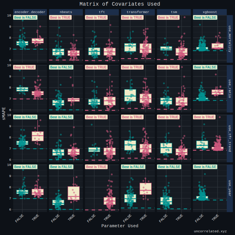
What about the static covariates? NIQ, latitude longitude? As we can see here, for the models that could process static covariates, their use was often deleterious.
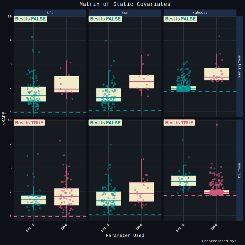
However, it can be seen that, during the hyperparameter tuning process models with NIQ were tested far more often than models with latitude longitude, suggesting that NIQ was superior to including the country’s position.
Input Window
As a reminder, the input window is simply the length of historical data a model uses to make its predictions. For example, if predicting tomorrow’s weather, a 7-day input window means the model only looks at the past week’s data to make its forecast.
This is a parameter we tuned. As you can see here, the results are mixed.
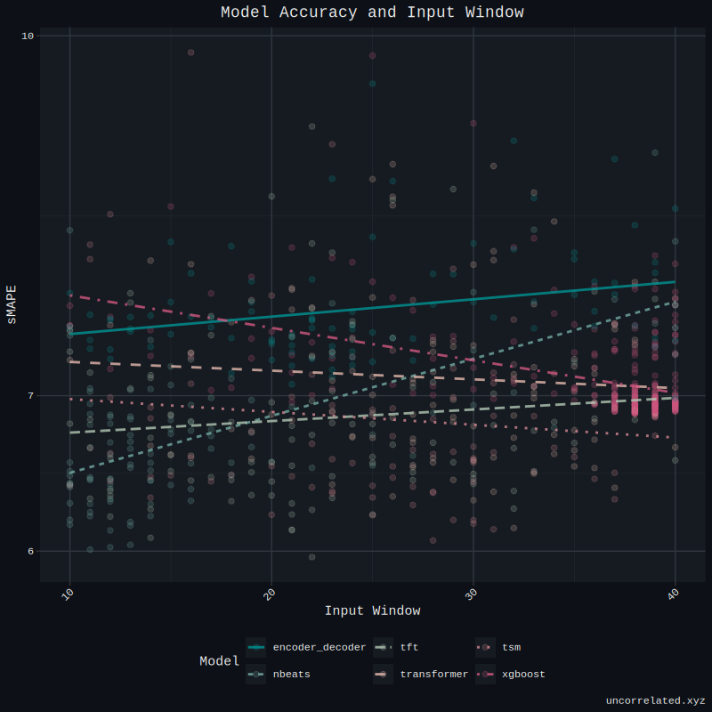
For some models, the longest possible window produced the best results, for others, the shortest. Overall, there wasn’t a significantly discernible effect in turning the input window.
Minimum Year
The minimum year in this case is the minimum year for data included in the set. Said another way, any data included in our dataset before the set minimum year is excluded. We turned this in our hyperparameter tuning process, as I was curious to see if inclusion of older data could benefit the models. The results was a strong yes, but only to a threshold point. To visualize this, a piecewise regression was made.
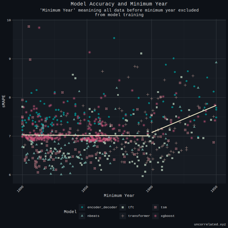
It seems that the inclusion of 19th century data has no effect on improving the quality of any of the models. However, the inclusion of the first half of the 20th century, notably the baby boom, did significantly improve model accuracy! We can see here that the correlation between minimum year and sMAPE is significant for models trained after 1900.
  term        estimate std.error statistic  p.value
  <chr>          <dbl>     <dbl>     <dbl>    <dbl>
1 (Intercept) -19.5      6.93        -2.82 0.00560
2 min_year      0.0140   0.00361      3.88 0.000166
This is important since, critically, the UN only bases their projections on fertility data for 1950 onward.
Forecasts: Apples to Apples
Now we need to compare results to the UN’s models. To do this, we must be as “apples to apples” as possible. This means doing the following:
- Test both the UN’s and our models on unseen data.
- Make sure the data quality the UN’s model is based on is of comparable quality to ours.
Point two here is the most important. We’re going to be testing our projections against the UN’s 2013 forecasts. Our models will not have access to, or be trained on data from 2013 onward to make this comparison. However, note the data quality issues of the UN. For many countries, present TFR, or TFR for the past many years isn’t known.
Since we don’t have access to UN data quality/quantity records in 2013, we can’t know which countries for which they had to “guess” (project) what the present fertility was in 2013. If we assumed that the UN had access to complete data to 2013 this would be unfair. Because the UN’s 2013 model would in effect would actually be projecting further into the future than our model, if we were to test it on the next 10 years.
There are two ways to ameliorate this.
- We don’t use the UN’s 2013 projections, we directly replicate their methods from their github repo producing our own projections with the now complete data up to 2013 that we have today in 2024.
Or alternatively,
- We take the easiest approach, we only compare the UN’s projections against our own on countries that have the highest quality of record keeping.
I decided to take option two, since it was the easiest.
The results were the following for nearly 32 countries. Once again, accuracy is measured using sMAPE.
  model                mean median
  <chr>               <dbl>  <dbl>
1 nbeats_multivariate  6.87   4.11 }
2 tft_multivariate     7.39   4.88 } <- Ours
3 tft_simple           7.61   5.57 }
4 nbeats_simple        7.74   5.11 }
5 tfr_2013            11.7    8.97 <- UN
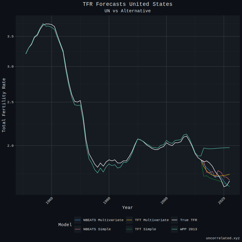
So compared to the UN’s forecasts from 2013, our best models yielded a substantial improvement. We can see this for the United States. Our models successfully forecast the declines in US TFR to the present day.
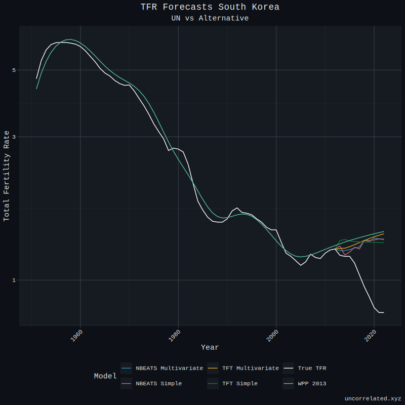
However, some forecasts still elude us. For example, South Korea has not improved much, if at all. We will touch on what can be done to solve this problem in the conclusion.
Final Forecasts: To the End of the Century
Now, the forecasts you’ve all been waiting for! The accurate forecasts to the end of the century, and beyond! Finally UN BTFO!

What’s this?
The above is a my live reaction after plotting the data. It isn’t pretty. Well, in all seriousness, it really isn’t that bad, but there are severe problems.
The forecasts into the immediate future were not accurate from the models we’ve trained on the full set. They suffered from the same problems as the UN - they regressed towards a mean quite quickly then maintained forecast. I’m disappointed to say this, but it failed somewhat.
Retrospective and Future Directions
So what went wrong, and what can be done to fix it so we can get forecasts to 2100?
Firstly, not using a test set. There is a mild tendency for overfitting to occur when doing this scale of hyperparameter tuning without a test set. This does make the validation results rosier than expected. Again - only to a very mild extent.
Secondly, the challenge of forecasting fertility rates, particularly in countries like South Korea experiencing historically low TFR, may stem from attempting to predict values outside the historical training data boundaries.
Several potential approaches could address this limitation:
Differential Modeling
Instead of directly predicting fertility rates, we could model the change in fertility rates over time. I did some initial testing of this approach. There was no logistic relationship between the classification of the differential model outperforming the non-differential model across TFR. In layman’s terms differential model didn’t do any better when TFR was lower. However, there seemed to be a very large improvement just at for the few countries with the lowest fertility rates.
Limit Transfer Learning
The current practice of pooling TFR all countries together for machine learning might be counterproductive. This approach should provide transfer learning, but country-specific patterns could be more important. A more nuanced approach would be developing individual models for each country, with training by country data weighted based on similarity in TFR, demographic indicators and socioeconomic factors. I actually already tested this - but not systemically and just for South Korea. The results seemed promising, the model was significantly more accurate.
This is where a test set is again useful - we could ensemble (combine) all of the above models. We could perhaps take this to an extreme and ensemble on a country by country basis, combining general and country-specific models. Although, I wouldn’t go too gung ho on this. The fact that using the year and lat/long failed to make its way into the model might suggest that this wouldn’t make a difference.
Why don’t I do this myself?
This was all time consuming. And, realistically, I doubt many folks will actually read this article. Most of the time I had to spend for this article was just learning the ropes of timeseries forecasting from the book and documentation I read. The coding didn’t take too long. In the future I would be interested in tackling this problem again, expanding the number of covariates analyzed, etc, applying different techniques and doing the due diligence of the test set. Finally, I would like to refine all this work, make a github repo and a benchmark for forecasting TFR; then update forecasts as new TFR data streams in.