Supplementary Materials

Downloads

Appendix

Frequently asked questions

Short answers for readers, and for anyone handing this supplement to an AI model to ask questions about the work. Details are in the sections that follow.

What was the question? Whether a current frontier AI, given a real survey respondent's record minus one test, can fill in that test: the person's total score, each item answer, the test's factor loadings and its population norms. The aim is imputing missing variables in survey datasets, not assessing individuals.

What data? Four public surveys: the General Social Survey (GSS), the National Longitudinal Surveys of Youth 1979 and 1997 (NLSY79, NLSY97) and Project Talent (1960 US high school students). The main benchmark has 106 targets: 80 multi-item tests and 26 single traits such as earnings or number of children (full list). A separate, private dataset of online personality, mental-health and IQ test responses, never published, was used as a replication sample.

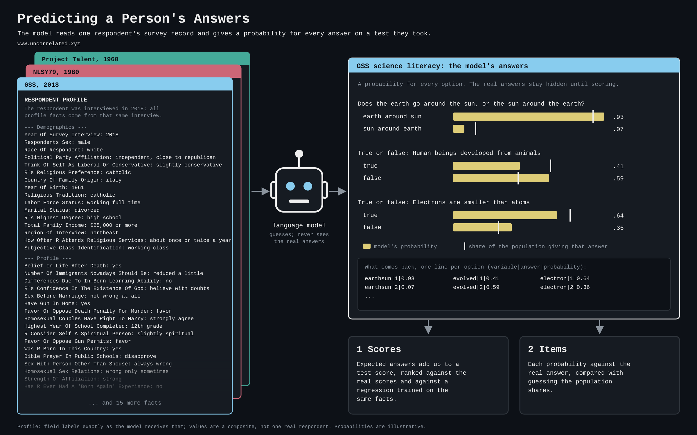
What exactly did the AI see? A short description of the study and the survey, the test's questions with every answer option and its code, an output format, and the respondent's profile: their other survey answers written as dated facts, one per line. It never saw the person's answers to the target test, any score derived from them, or any data from other respondents. The prompt opens:

You are taking part in a social science research study. Researchers are testing whether language models can predict how real people answered survey questions and tests in the General Social Survey (GSS), a nationally representative survey of US adults run since 1972. For each question below, estimate the probability that the respondent described at the end gave each possible answer, using only their profile.

It then gives the questions, asks for one line per answer option in the form variable|response_code|probability, tells the model to predict "this specific person, not an average person", and ends with the profile.

Which models, and when? Two waves. July to August 2026: Gemini 3 Flash through OpenRouter, used for the norms method, its AI personas and early rounds. September to October 2026: Opus 5.5 at medium reasoning effort, through Claude Code with tools disabled, one isolated call per person and test, prompts frozen before any call. Scores, Items, Loadings and the private-data replication use Opus 5.5; Norms and the cross-survey persona results use Gemini 3 Flash.

How was leakage handled? Each target has its own exclusion list: its own items, totals and equivalent scores, all cognitive scores when the target is an ability, and fields judged to give the answer away. A review pass followed. Proxies found later, such as party identification for political views, were removed and eight targets rerun on the same people; both versions are reported (Leaks). Historical Project Talent results from the first wave were run on profiles that still carried vocabulary scores, and are labelled as such.

What is the baseline? A ridge regression on exactly the same profile fields, trained on the survey's other respondents (thousands, with the real target values), excluding the 50 people being predicted. It is supervised; the AI is not. With 40 to 70 fields per test it is stronger than a conventional 12-variable regression.

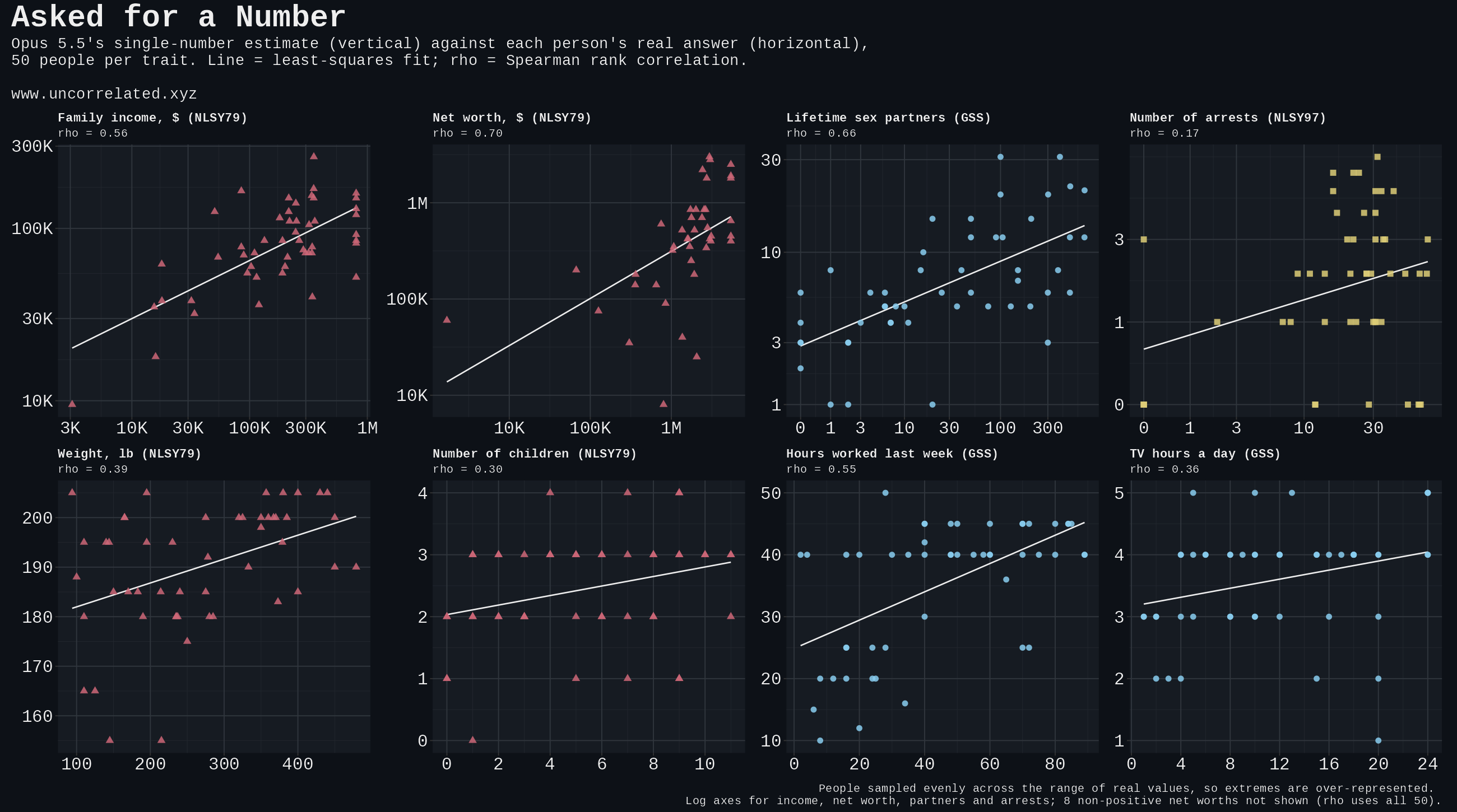
How big are the samples? 50 respondents per test, sampled evenly across real scores and reweighted to the population. Single tests are therefore noisy (a correlation of .5 has a standard error of about .1, more after reweighting), which is why the accuracy scatter removes sampling noise (Sampling noise). Private-data person-level tasks use 20 people per test.

Which metrics? They differ by section and should not be compared directly:

• Scores: population-weighted Pearson or Spearman correlation between predicted and real totals.
• Items: kappa (exact match corrected for chance) and log-loss skill over the population's answer shares.
• Loadings: Pearson correlation between elicited and actual one-factor loadings, signed and on size alone.
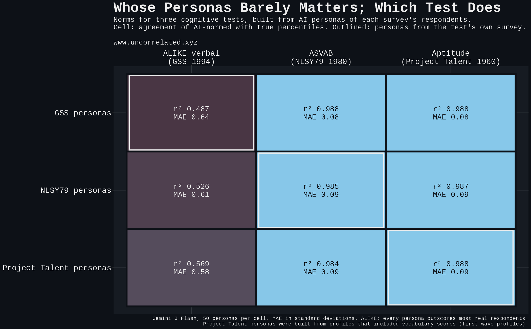
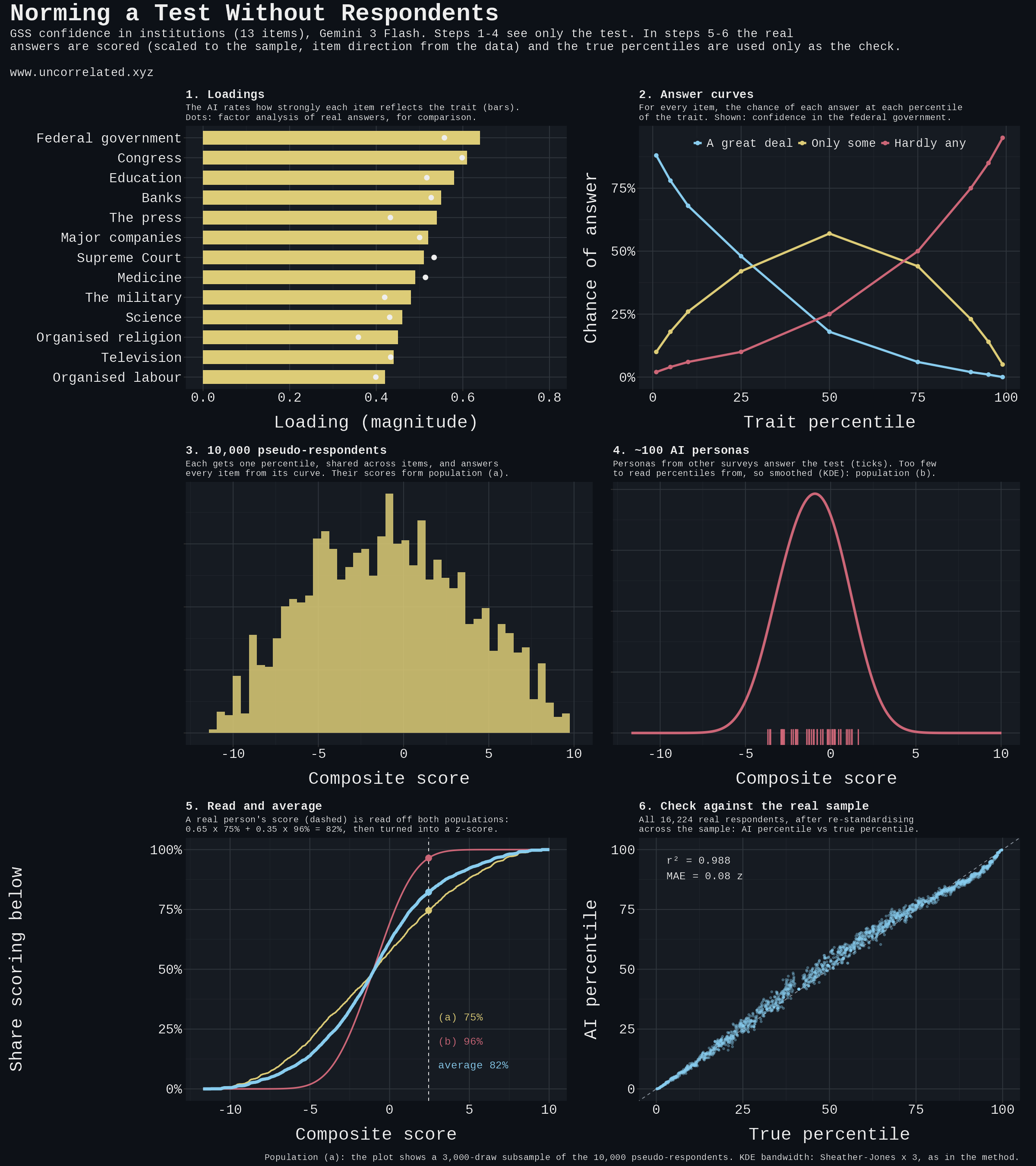
• Norms: squared Pearson correlation (r²) and mean absolute error, in standard deviations, between AI-normed and true percentiles.

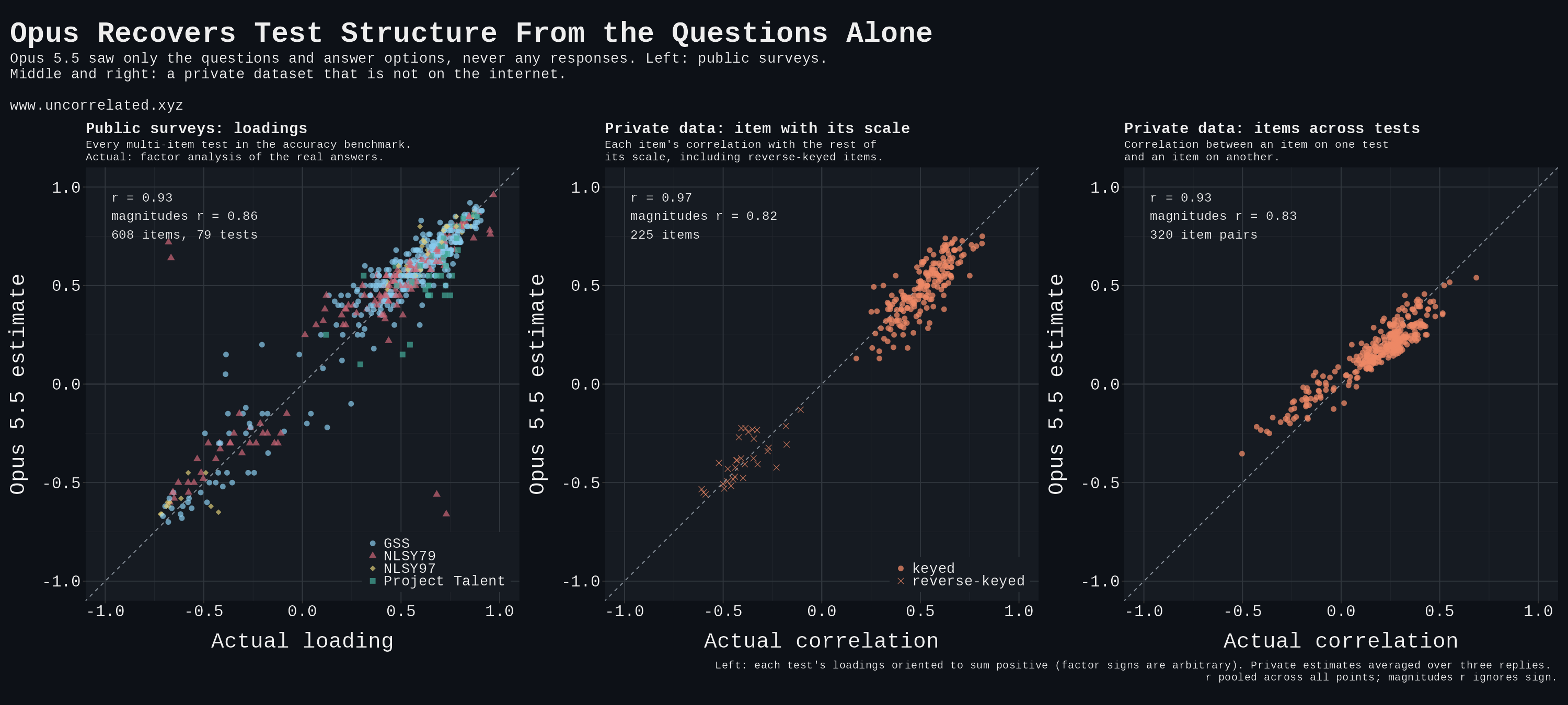
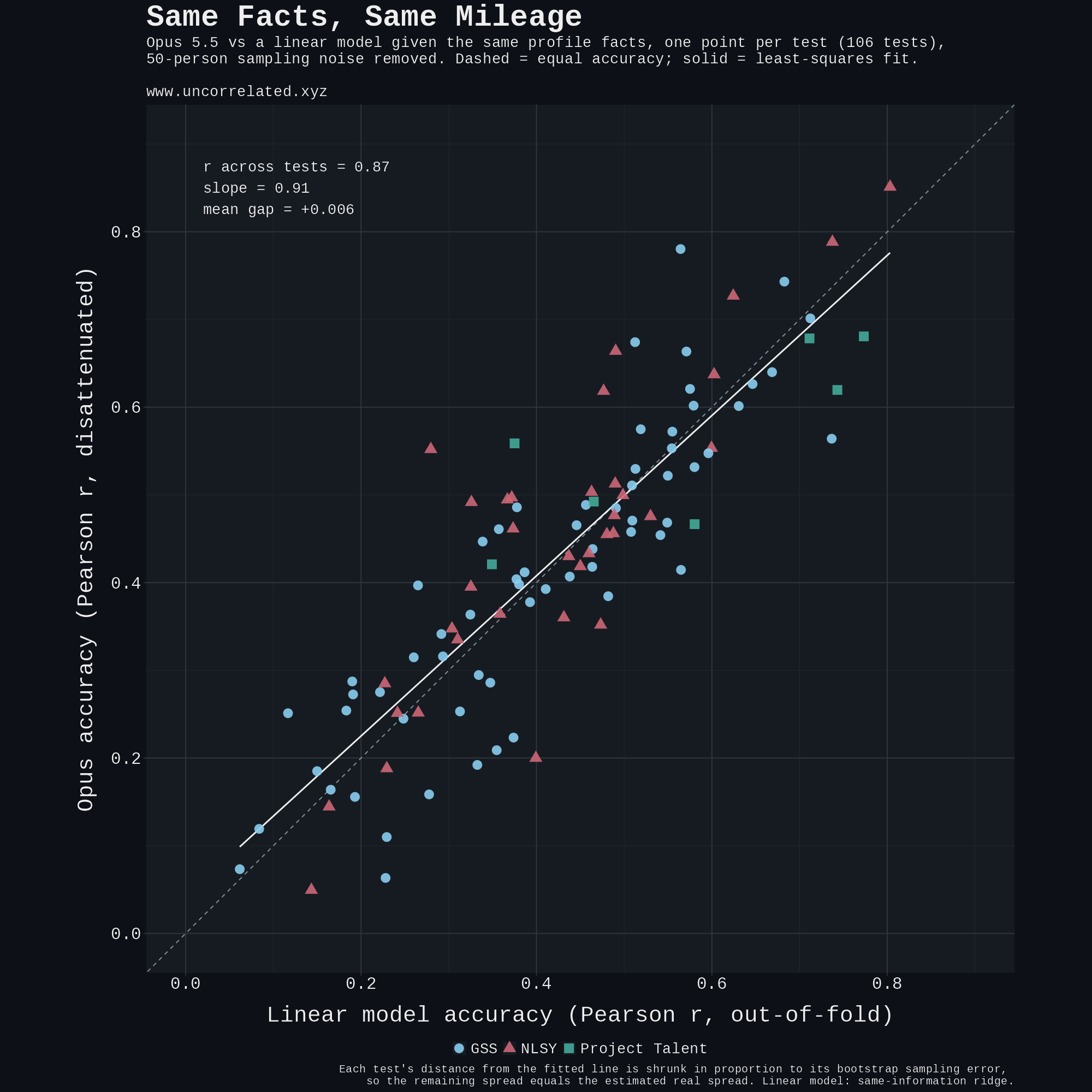
What is the main result? Opus and the ridge tie: mean Spearman .450 against .448 on 60 batteries. Across the 106 tests their accuracies correlate .87 once sampling noise is removed (slope .91): both do well where the profile is informative and fail where it is not. At the item level Opus's top answer is usually just the population's most common one (kappa .35, log-loss skill .02). From the questions alone it recovers loadings well (r .93 signed, .86 on size, 608 items).

Did the AI just remember the surveys? These surveys are public and widely analysed, so training exposure to their aggregates cannot be ruled out; individual respondents' records are much less likely to have been memorised, but that was not tested directly. The private dataset is the check: where its tasks match the public analyses, the results are similar (Replication).

Do the norms need any real data? Yes, in the form tested. The AI supplies loading sizes, answer curves by percentile and role-played respondents, but scoring the real people uses the real sample's item means, SDs and item directions, and the AI-normed percentiles are re-standardised across the real sample. With a full sample, simply ranking it beats the AI reference (mean r² .987 against .949). The case the method is meant for, norming a new test or a handful of takers with no sample, is untested.

Are imputed scores measurements of the trait? No. An imputed score carries the profile's information, not the trait's. It is a proxy, and anything built on it needs checking against independently measured outcomes, not against the imputed values themselves.

What is not claimed? That the AI reads individuals better than a regression on the same facts; that it measures intelligence; that its percentiles would hold without a reference sample; or that these results generalise beyond the four surveys, the private dataset and the models tested.

Method in detail

Profiles. Profiles are built per test from the respondent's own record, with facts from any survey wave labelled by year. A model (Opus 5.5) rated each candidate field for relevance to the target. A screen then removed the target's own items, its totals and equivalent scores, cognitive scores when the target is an ability, and fields flagged as giveaways, and a review pass flagged further giveaways, contradictions and duplicate lines before anything was frozen. Missing facts are simply absent from the profile. Each test's panel is 50 people with at least 30 profile facts, sampled evenly across the range of real scores so that both tails are represented; correlations are then reweighted to the population, because sampling evenly across scores inflates them.

Leakage. The screen removes the target's own items, its totals and equivalent scores, all cognitive scores when the target is an ability, and fields flagged as giveaways; a manual review pass follows. Proxies found after scoring were ablated and the affected tests rerun on the same people (see Leaks, and what they were worth).

Model. Opus 5.5 at medium reasoning effort, through Claude Code with tools disabled, one turn per person and test, and a fixed prompt with instructions first and the profile last. Each answer option gets a probability; numeric items are answered as probabilities over up to six ranges cut at published percentiles. Unparseable replies were excluded, never repaired (under 1%). The test's own scoring rule turns the expected item answers into a total. Variants that also showed the population answer rates, or the full scoring key and item statistics, did not improve ranking.

Baseline. Ridge regression on the rendered profile facts: numeric facts as numbers, categorical facts as indicators, missing values mean-filled with a missing-value indicator, and the penalty chosen by cross-validation. It is fitted on the survey's reference sample (thousands of labelled respondents, excluding the panel) and applied to the panel. It has the labels the model lacks and nothing else. With 40 to 70 fields per test it is a generous baseline by the standards of a conventional 12-variable model.

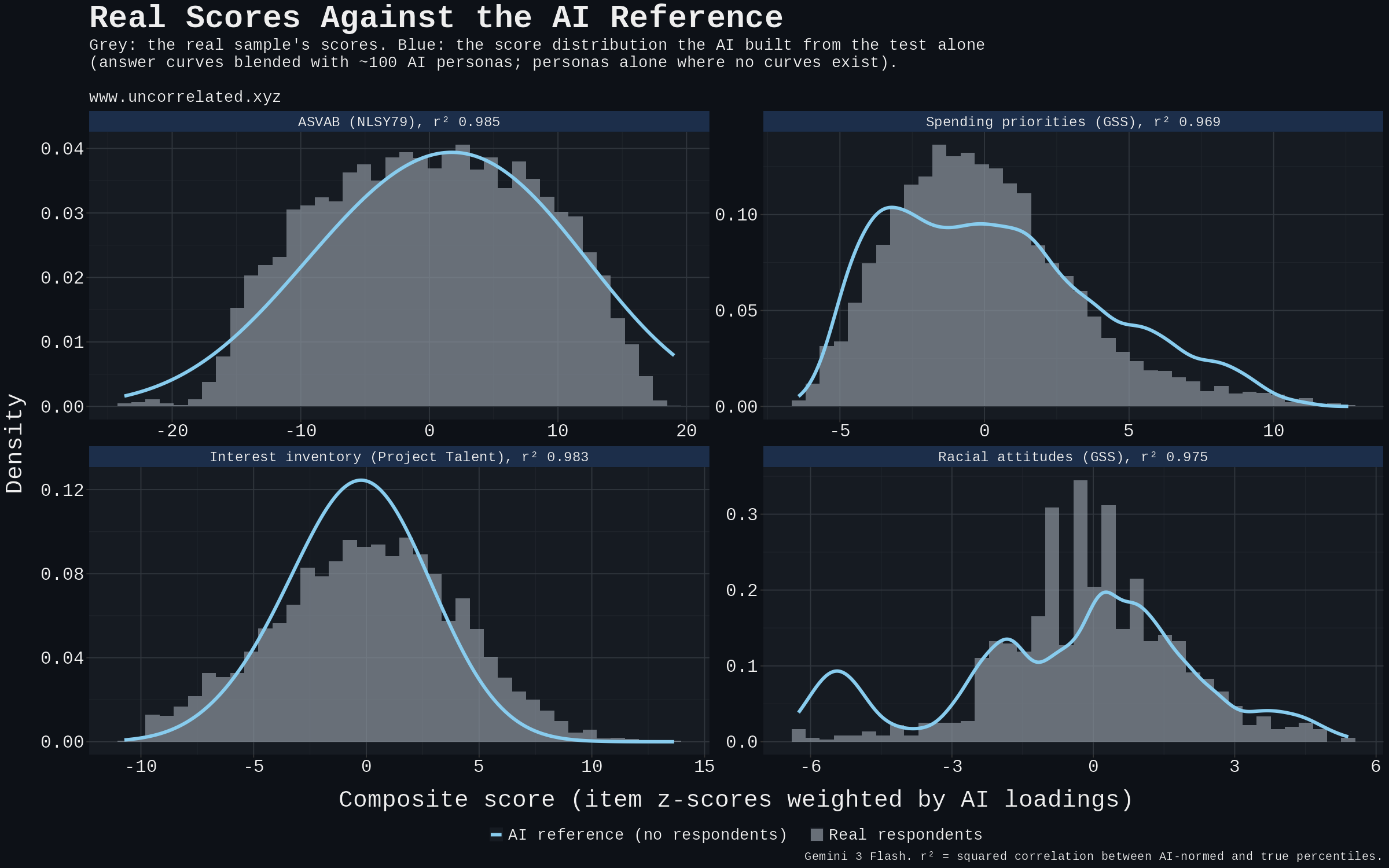
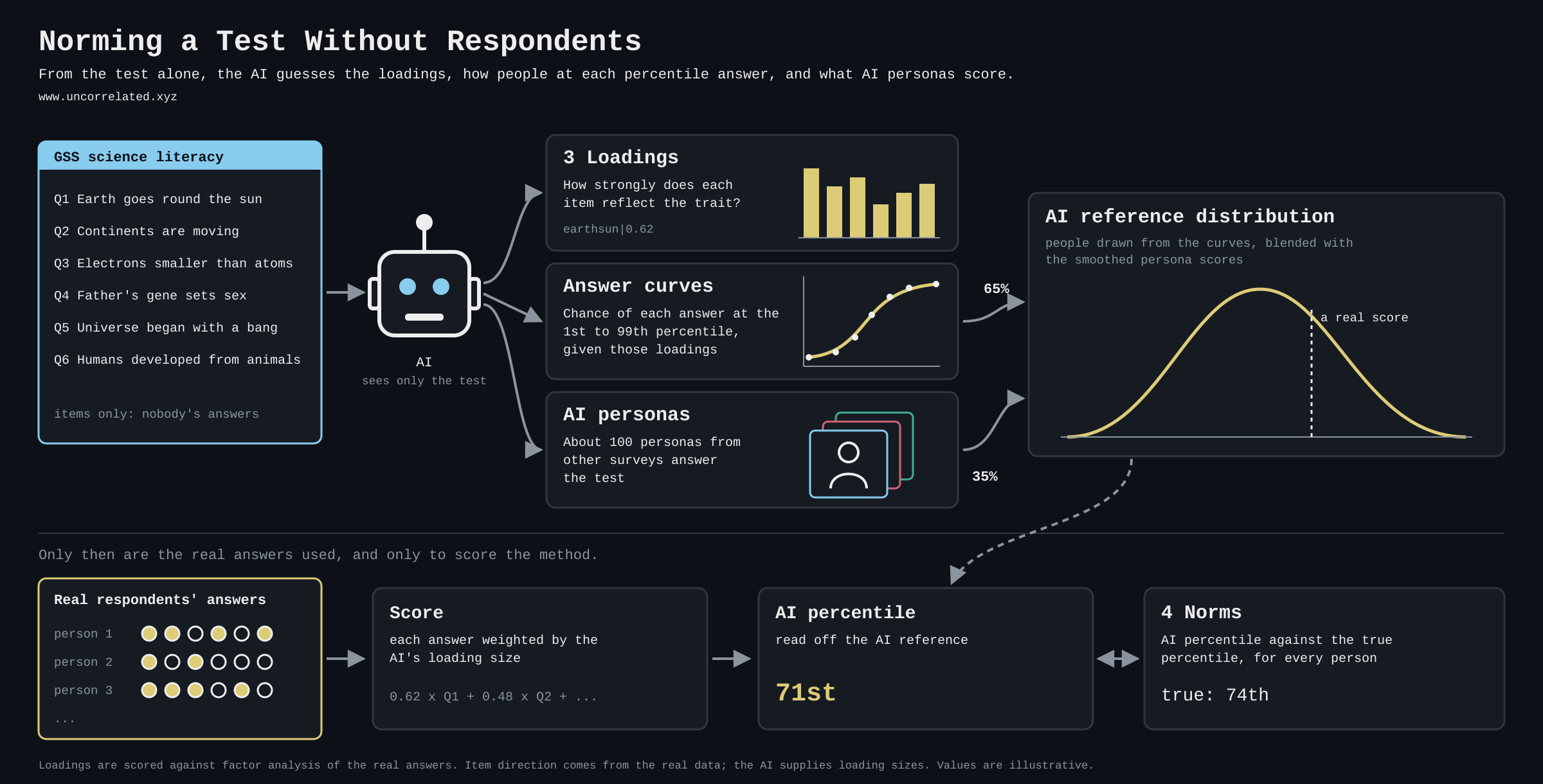
Norms reference curve. Real respondents' item answers are scored into a loadings-weighted composite. The reference curve blends a Monte Carlo distribution built from the model's estimated answer curves per percentile (65%) with a smoothed density over about 100 role-played respondents' composites (35%). Norm quality is the squared Pearson correlation between each person's AI-normed and true percentile, as z-scores, a different metric from every other number in this post. Scoring uses the real items' means, SDs and keying, and the AI-normed z-scores are re-standardised across the real sample (mean 0, rank-implied SD), so not every step is free of target data. The CDF readings are averaged 65/35 (chosen by leave-one-battery-out selection), with KDE bandwidth Sheather-Jones × 3. On the same batteries, ranking the sample on the AI-weighted composite gives mean R² .987 and mean absolute error .065 z, against .949 and .156 for the AI reference.

The 106 benchmark targets

Each target was predicted for the same 50 respondents by Opus 5.5 and by the ridge regression. All values are population-weighted Pearson correlations between predicted and real totals. "Ridge, same panel" scores the ridge on those 50 people, as in the post's intelligence table; "Ridge, reference sample" is its out-of-fold correlation in the full labelled sample, the horizontal axis of the post's accuracy scatter. Differences between the two ridge columns come from the panels' small size and their sampling evenly across scores. † Rerun without fields later found to restate the target (see Leaks, and what they were worth). Within each group, targets are sorted by Opus's correlation.

Cognitive ability and knowledge (13)

Target	Survey	Opus 5.5 (r)	Ridge, same panel (r)	Ridge, reference sample (r)
ASVAB, 1980	NLSY79	.86	.81	.80
CAT-ASVAB, 1997–98	NLSY97	.80	.72	.74
Cognitive screening: orientation, 2020	NLSY79	.68	.60	.28
Aptitude tests, 1960	Project Talent	.68	.77	.71
Information Test, Part I, 1960	Project Talent	.66	.82	.77
Science knowledge quiz	GSS	.63	.65	.65
WORDSUM vocabulary test	GSS	.62	.63	.58
Cognitive screening: counting backwards, 2020	NLSY79	.58	.66	.33
Information Test, Part II, 1960	Project Talent	.57	.68	.74
Verbal fluency (animal naming), 2018	NLSY79	.56	.57	.37
Knowledge of the World of Work, 1979	NLSY79	.53	.52	.60
Environmental knowledge quiz	GSS	.38	.45	.41
ALIKE verbal similarities test	GSS	.32	.33	.48

Personality, self-concept and wellbeing (30)

Target	Survey	Opus 5.5 (r)	Ridge, same panel (r)	Ridge, reference sample (r)
Daily spiritual experiences	GSS	.76	.70	.68
SF-12 health items, age-60 module	NLSY79	.66	.63	.60
Self-reported delinquency, 1997	NLSY97	.57	.23	.37
Rosenberg self-esteem, 1987	NLSY79	.55	.51	.46
K6 psychological distress	GSS	.54	.37	.38
Religious belief and practice, 2011 †	NLSY97	.53	.51	.49
Empathic concern	GSS	.52	.60	.34
Interest inventory, 1960	Project Talent	.51	.65	.47
CES-D short form, age-50 module	NLSY79	.51	.48	.50
MHI-5 mental health, 2010	NLSY97	.50	.52	.37
PROMIS global health	GSS	.50	.46	.46
Rosenberg self-esteem, 1980	NLSY79	.47	.45	.49
Self-rated internet skills	GSS	.45	.53	.39
Misanthropy (trust in people)	GSS	.45	.50	.51
Religious belief and practice, 2017 †	NLSY97	.44	.46	.48
MHI-5 mental health, 2015	NLSY97	.44	.43	.33
MHI-5 mental health, 2008	NLSY97	.42	.41	.46
Rosenberg self-esteem (GSS)	GSS	.42	.37	.51
Anomia	GSS	.41	.39	.54
CES-D short form, 2022	NLSY79	.40	.52	.49
Temperament inventory, 1960	Project Talent	.40	.59	.58
Self-rated knowledge of topics	GSS	.37	.49	.39
CES-D depression, 1992	NLSY79	.37	.34	.36
MHI-5 mental health, 2000	NLSY97	.34	.35	.31
Pearlin mastery, 1992	NLSY79	.31	.34	.43
Rotter locus of control, 1979	NLSY79	.23	.36	.27
Images of God	GSS	.19	.34	.31
Altruistic love	GSS	.18	.47	.35
Attitudes to school, 1979	NLSY79	.11	−.01	.16
Satisfaction with areas of life	GSS	.03	.27	.35

Social and political attitudes (29)

Target	Survey	Opus 5.5 (r)	Ridge, same panel (r)	Ridge, reference sample (r)
Abortion: willingness to help	GSS	.82	.77	.56
National spending priorities	GSS	.69	.66	.57
Women's roles, 1982	NLSY79	.66	.66	.48
Environment module, 2021	GSS	.64	.61	.67
What makes someone truly American	GSS	.60	.68	.63
Government responsibility (ISSP)	GSS	.59	.55	.55
Civil liberties (tolerance of unpopular views) †	GSS	.55	.61	.51
Government responsibility (1–5 scale)	GSS	.52	.48	.58
Globalism (national identity module)	GSS	.49	.45	.49
Environmental worldview (ISSP)	GSS	.48	.51	.45
Abortion: legal grounds	GSS	.44	.47	.74
What matters in a democracy	GSS	.43	.49	.38
Gender roles	GSS	.42	.61	.46
Racial attitudes	GSS	.42	.36	.55
Attitudes to science	GSS	.36	.44	.26
Warmth towards racial groups	GSS	.33	.37	.29
Attitudes to children's mental-health medication	GSS	.33	.18	.19
Influences on children	GSS	.30	.32	.22
Women's roles, 1979	NLSY79	.27	.45	.47
Perceived social conflict	GSS	.26	.20	.33
Terrorism preparedness	GSS	.23	.32	.25
Attitudes to doctors	GSS	.20	.18	.15
Fairness of groups	GSS	.12	.12	.08
Confidence in institutions	GSS	.11	.25	.37
Attitudes to psychiatric medication	GSS	.11	.30	.19
Adults' roles in children's lives	GSS	.05	−.07	.06
Contributions of ethnic and religious groups	GSS	.05	.41	.33
Interest in the International Polar Year	GSS	.02	.28	.28
Government security measures	GSS	−.02	.07	.23

Work (8)

Target	Survey	Opus 5.5 (r)	Ridge, same panel (r)	Ridge, reference sample (r)
Job rewards (ISSP)	GSS	.71	.70	.51
Work–family conflict	GSS	.48	.41	.26
Job rewards (Quality of Worklife)	GSS	.34	.32	.19
Job satisfaction, 1981	NLSY79	.33	.19	.23
Refusing work for family reasons	GSS	.32	.15	.12
Job satisfaction, 1979	NLSY79	.14	.16	.23
Workplace safety climate	GSS	.14	.28	.17
Workplace climate and trust	GSS	−.17	−.03	.23

Single traits (26)

Target	Survey	Opus 5.5 (r)	Ridge, same panel (r)	Ridge, reference sample (r)
Highest degree, 2023	NLSY97	.76	.80	.62
Net worth, 2016	NLSY79	.73	.72	.49
Religious attendance	GSS	.71	.76	.71
Years of schooling	GSS	.64	.65	.58
Dating frequency, 1960	Project Talent	.63	.53	.38
Sex partners, last five years †	GSS	.61	.62	.52
Number of children (GSS)	GSS	.56	.54	.55
Frequency of sex	GSS	.52	.62	.60
Own earnings †	GSS	.52	.54	.51
Political views †	GSS	.52	.52	.55
Hours worked last week	GSS	.51	.53	.36
Study hours a week, 1960	Project Talent	.45	.49	.35
Family income, 2019	NLSY79	.45	.51	.53
Number of children (NLSY79)	NLSY79	.43	.31	.44
Self-rated health	GSS	.41	.50	.38
Gun in the home †	GSS	.39	.37	.46
General happiness	GSS	.39	.37	.32
Number of arrests	NLSY97	.39	.48	.45
Hours of television a day	GSS	.38	.37	.44
Smoked in the past year	NLSY97	.37	.48	.30
Lifetime sex partners	GSS	.35	.34	.29
Occupational prestige	GSS	.31	.41	.56
Sexual orientation	GSS	.29	.19	.18
Sex partners, 2003	NLSY97	.25	.26	.24
Weight, 2018	NLSY79	−.09	.14	.40
Drinking days, last month	NLSY97	−.12	−.12	.14

Leaks, and what they were worth

Some profile fields that passed the automatic screens were, on inspection, near-restatements of the target: views on homosexuality in a civil-liberties scale, party identification for political views, stated religion for religiosity, family income for earnings. Rerunning those 8 tests on the same people without the offending fields, Opus fell by .08 on average and the ridge by .06 (religiosity alone fell .15 to .19). Opus minus ridge moved from +.02 to .00. The leaks helped both about equally, so they inflated accuracy without changing the comparison.

Sampling noise in the accuracy scatter

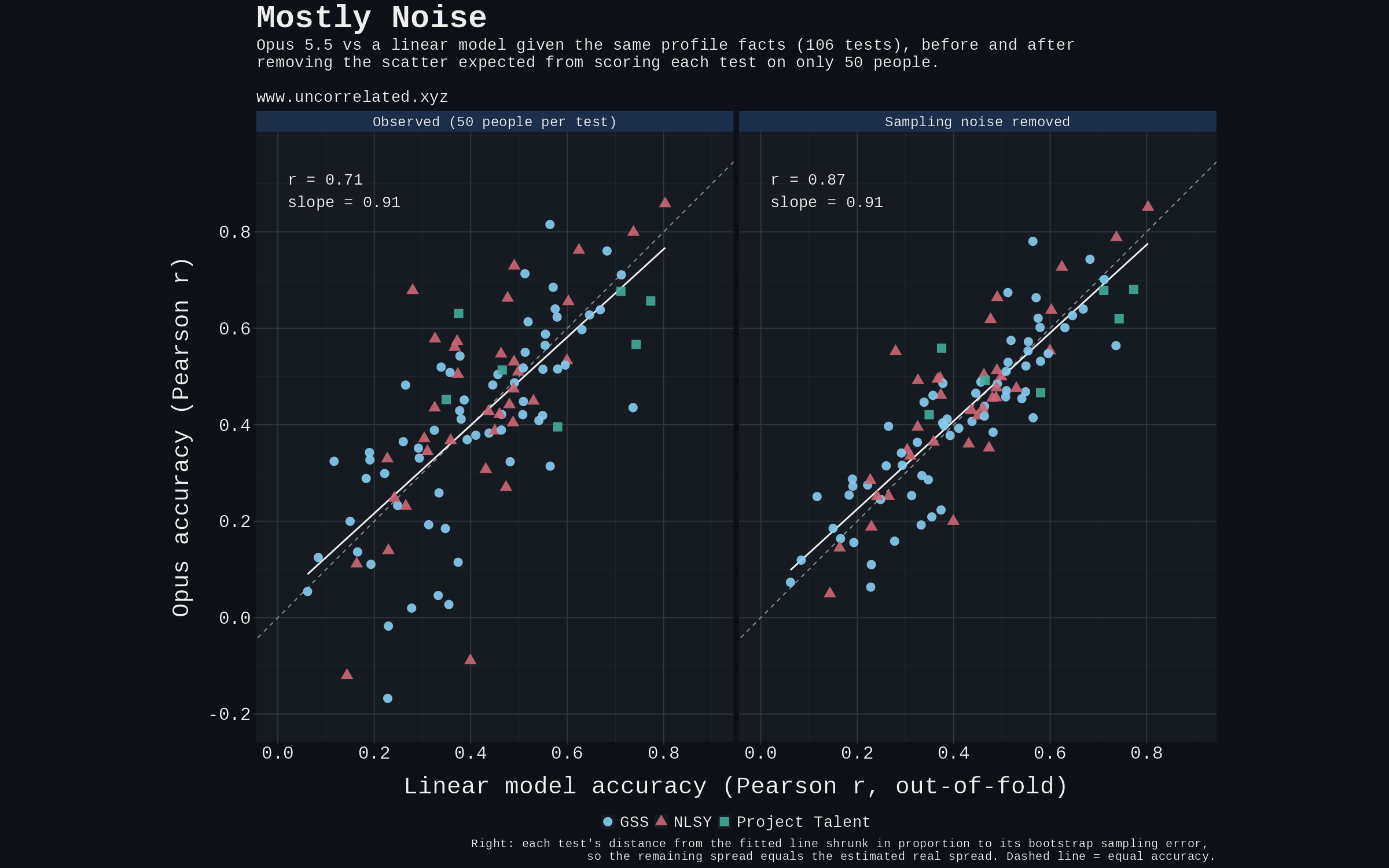
With 50 people per test, each test's correlation has a standard error of about .1. Bootstrapping the panels shows that about two-thirds of the spread around the line is what 50-person samples alone would produce. For each test, bootstrapping its 50 people 2,000 times gives the sampling variance of Opus's r. The scatter around the fitted line has variance .022; the average sampling variance is .015, about two-thirds of it, leaving a real spread of about .08 in r between tests. Correcting the across-test correlation for that unreliability gives about .88; the right panel shrinks each test toward the line in proportion to its sampling error. This .88 is a correlation between two accuracies across tests, not a prediction accuracy, so it is not comparable with the experiment-prediction figures in the post.

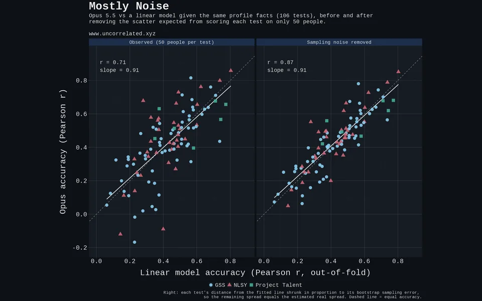Figure S1. The accuracy scatter before and after removing 50-person sampling noise.

Earlier rounds

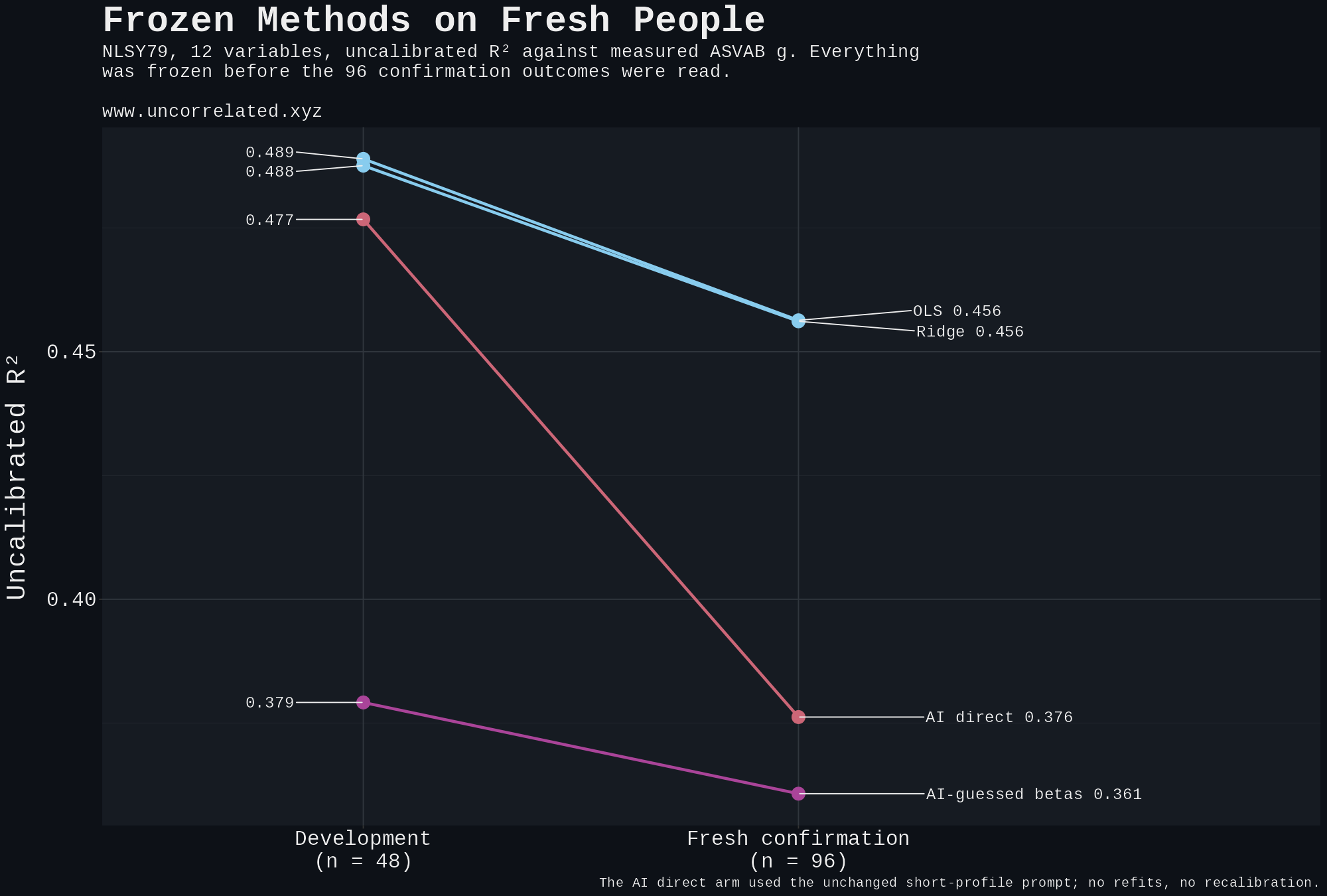
Earlier rounds with a cheaper model and shorter profiles told the same story with more noise. On NLSY79, Gemini 3.8 Flash reading 12 fields nearly matched a 12-variable regression on 48 development people (uncalibrated R² .477 against .489) but slipped on 96 fresh people (.376 against .456). On Project Talent, once vocabulary-related context was removed from the profiles, it collapsed (R² .028 against .244). Every earlier Project Talent result that looked better had that vocabulary anchor in the profile.

These are uncalibrated R² (1 − SSE/SST on raw predictions), a different metric from the correlations in the post. Development: 48 people; confirmation: 96 different people, with predictions frozen before scoring. The 12 predictors were 1979 variables chosen by hand, with no cognitive context.

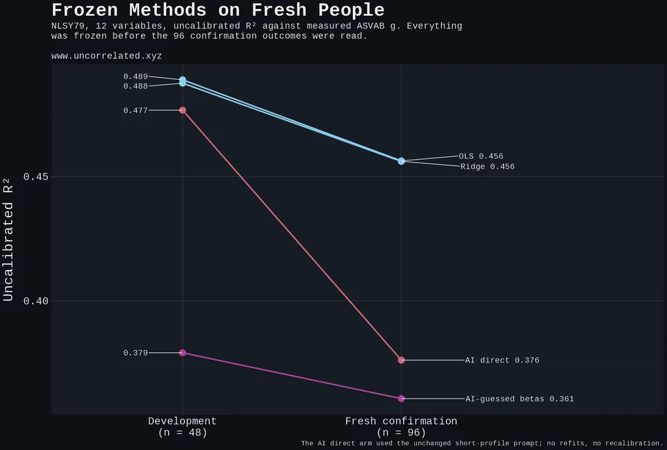Figure S2. NLSY79 development against fresh confirmation people, Gemini 3.8 Flash, uncalibrated R².

Order within batteries of separate items

On batteries of separate items (feeling thermometers, music tastes), Opus orders a person's answers no better than the population average order (.57 against .57), with music and thermometers the exceptions.

Drawing imputed answers

Drawing imputed answers is its own problem. Independent draws from the item probabilities keep too little spread and almost none of the correlation between items (real inter-item correlation .19, one imputed draw about .04), so 95% intervals for the total cover the truth only 75% of the time. Adding one shared latent term per person, tuned only to the published total SD, restores coverage to about 90%.

Loadings by battery, and the personas' trait correlations

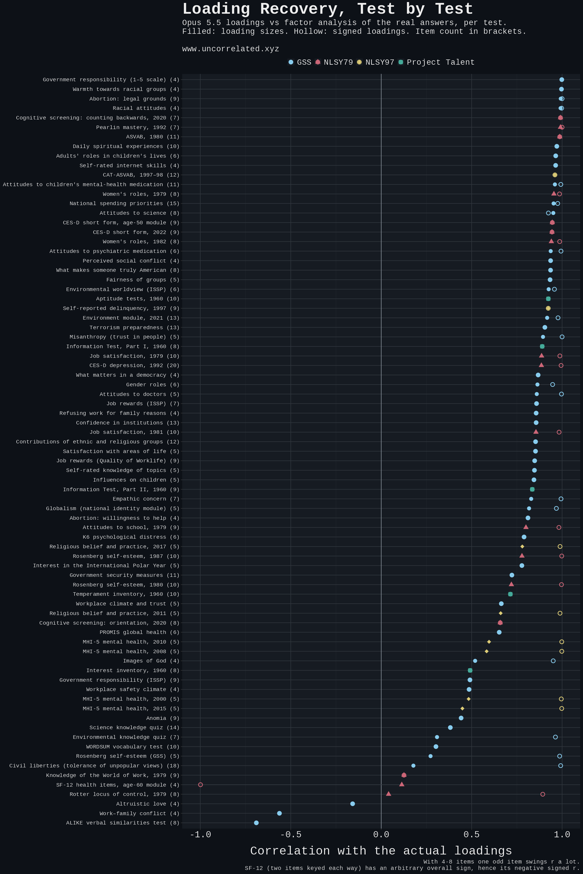
Within a test, Opus's loading sizes correlate with the real ones at a median of .85 across the 79 tests (middle half .62 to .94). Signed loadings do better, because getting the direction of keying right is easy. The ASVAB is near perfect (.99 on size, CAT-ASVAB .96). The weakest tests mostly have items that load about equally (SD of actual loadings .03 to .10, against a median of .11), which leaves little for a correlation to find: ALIKE, work–family conflict, altruistic love, Rotter locus of control, the SF-12 items and Knowledge of the World of Work.

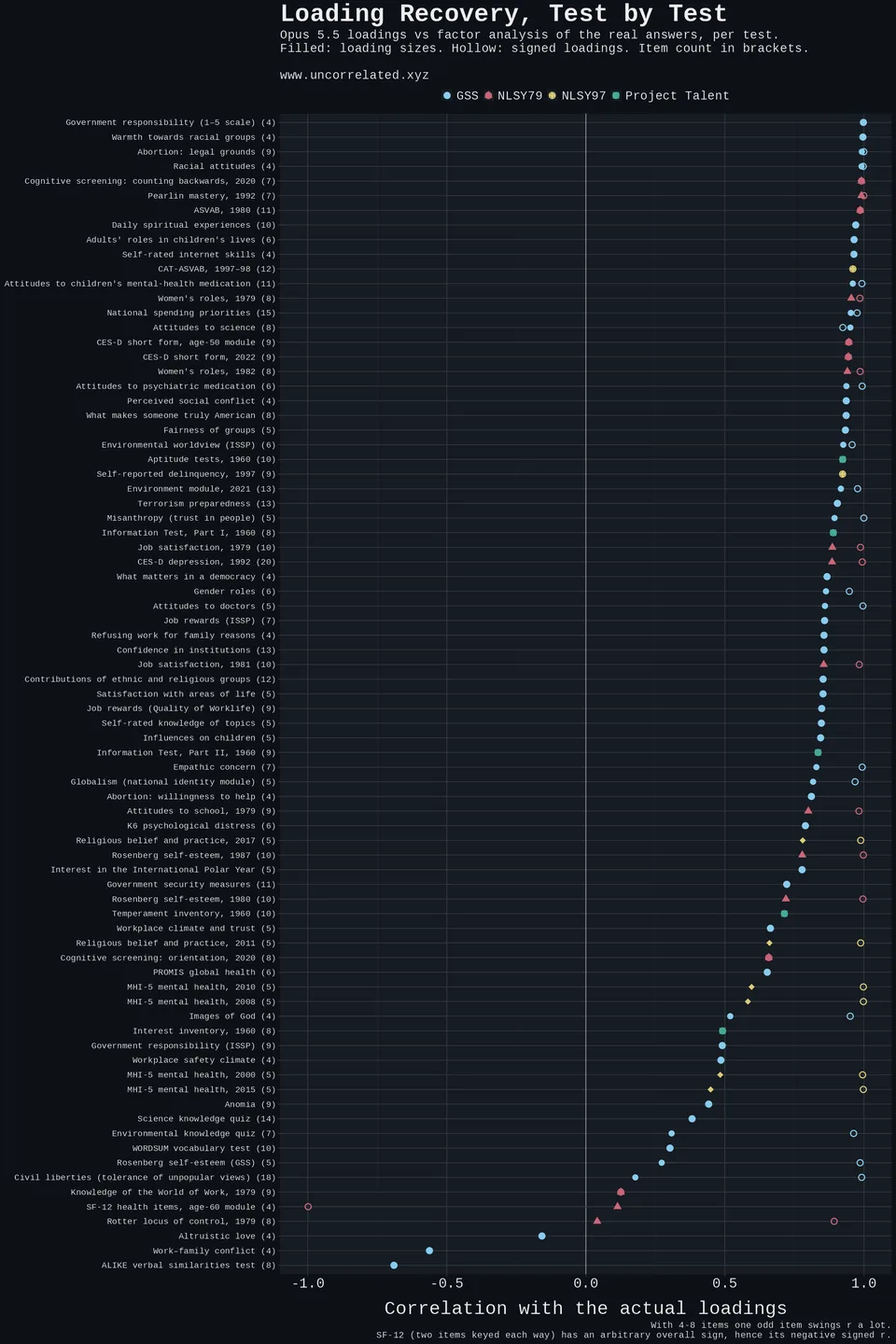Figure S3. Opus 5.5's loading recovery within each test, on size (filled) and signed (hollow).

In the earlier Gemini 3 Flash runs, the AI's personas got the broad structure but not the size. Correlations between traits in their answers tracked the real correlations (r = .82) but came out about twice as strong: the personas were more internally consistent than real people.

Norms by battery

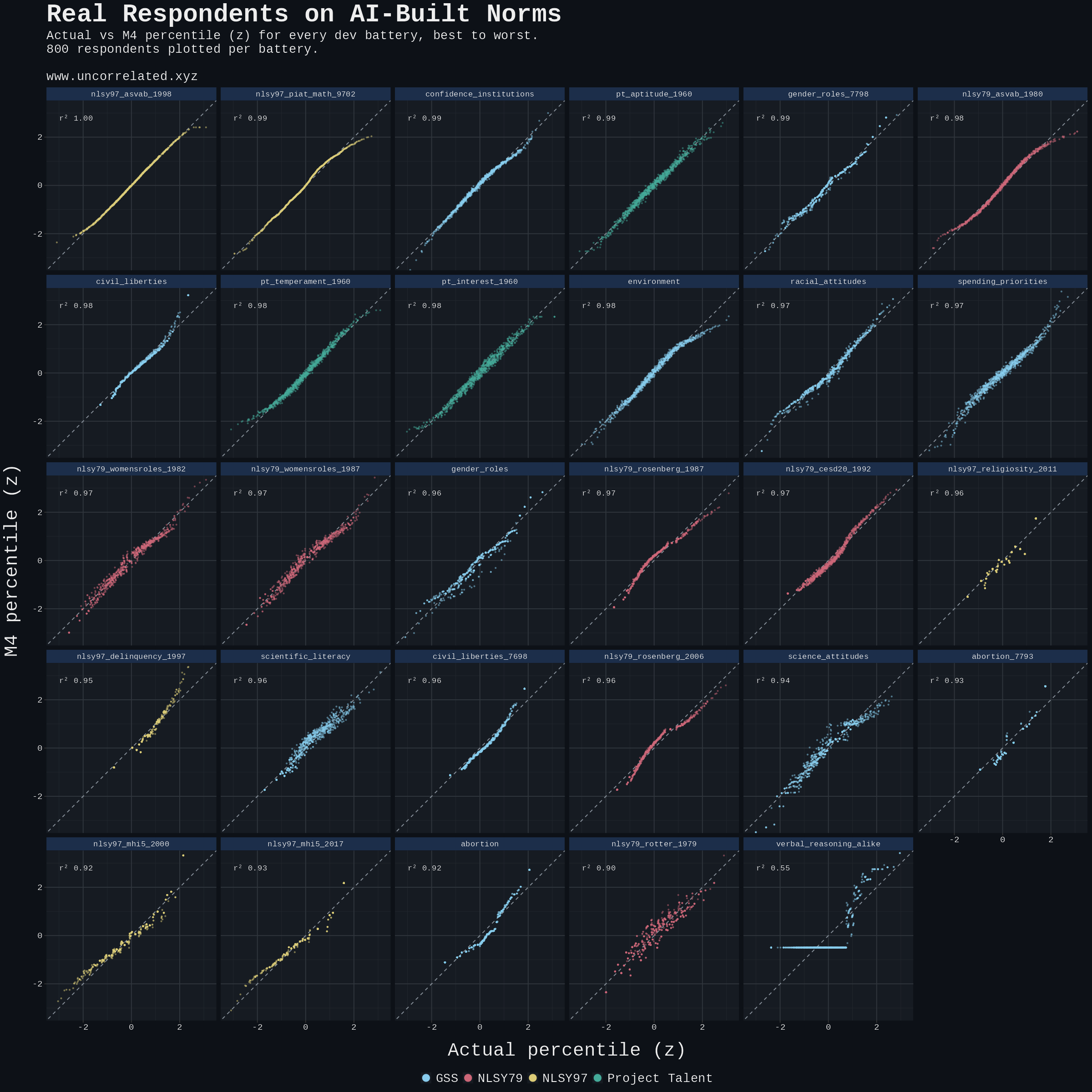
AI-normed against true percentile for each of the 29 development batteries (Gemini 3 Flash). The single failure is ALIKE, where every AI persona outscores most real respondents and the bottom 60% of real people are squashed onto the bottom of the reference curve.

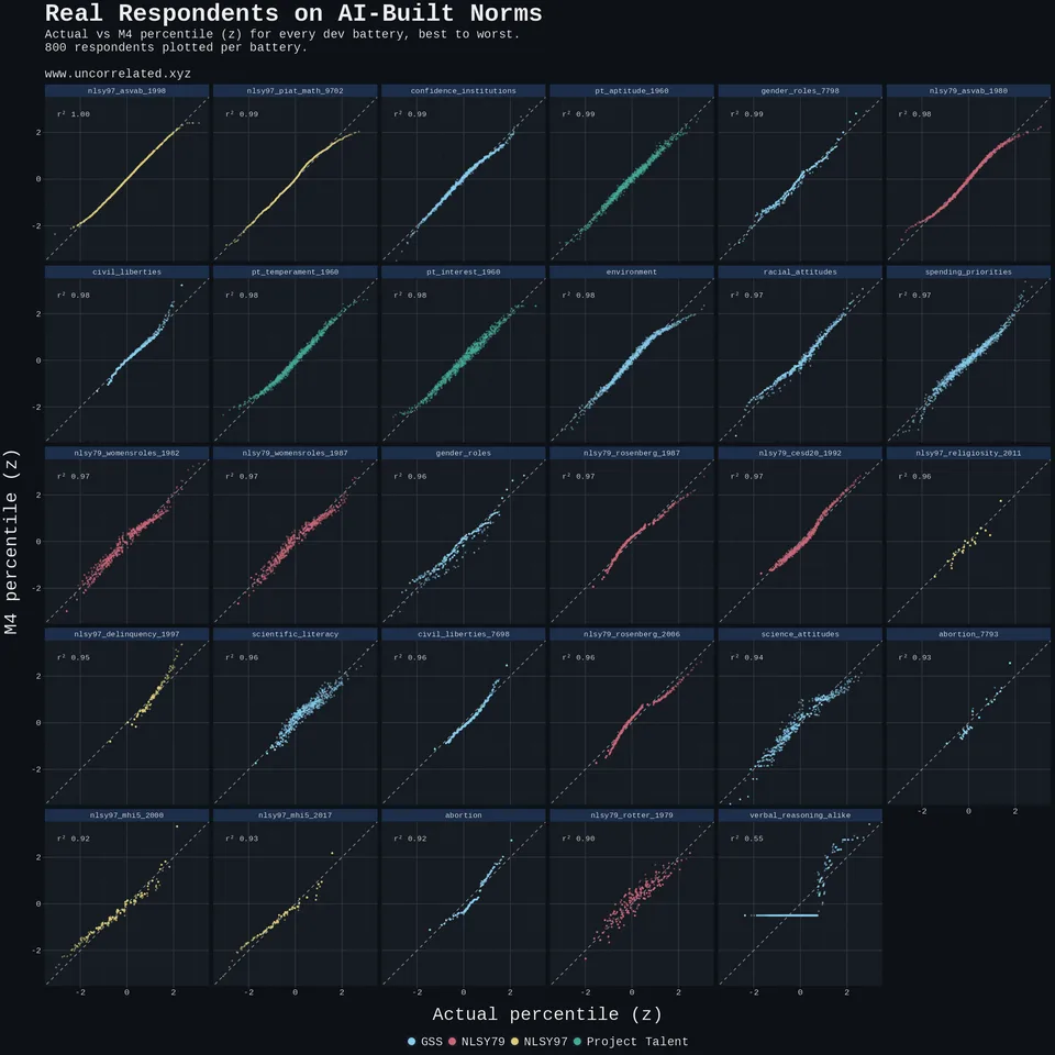Figure S4. AI-normed against true percentile for each development battery, Gemini 3 Flash.

Notes on the stereotype evidence

Accuracy here is correspondence: the correlation between perceived and actual values across groups or attributes. Consensual accuracy uses the average perceiver; personal accuracy scores each perceiver separately. Jussim's convention counts r ≥ .40 as accurate and .25 to .40 as moderately accurate, against a field where about 5% of effects exceed r = .50 (Jussim et al., 2009). His tallies are a non-systematic review by the programme's main proponent, and the numbers for some studies differ between versions, so the post's table uses primary studies wherever they were available. The main critique is that many stereotypes are generic beliefs ("X are Y") rather than statistical estimates, and generics need not track statistics even when percentage estimates do (Jussim, 2015). Whether AI behaves as a statistical estimator or a store of generics is untested, and the answer may depend on how you ask.

Three of the four papers from this group appeared in OpenPsych journals, which use open forum review and which Kirkegaard co-founded; the fiscal-contribution study appeared in Societies (MDPI). In their favour: preregistration, planned samples, public data, confidence intervals, and a preregistered numerical prediction (r = .84) that was met (.81). Against: one research group, and in the 2016 study the exclusion rules were extended after data collection began, including a rule that removed respondents whose own accuracy was below r = −.20, which inflates the individual figures. A related UK paper correlates opposition to immigration with arrest rates across 23 nationalities (r = .69), but it measures attitudes rather than beliefs and divides London arrests by UK-wide populations (Carl, 2016). The apparent errors for Muslim-majority groups, underestimated benefit use in one study and overestimated fiscal contribution in another, may be regression toward the mean, as the 2020 paper itself notes.

Notes on the cited AI studies

Ashokkumar et al. Figures from the PsyArXiv preprint; the Nature version was not available to check. An earlier working-paper version is widely quoted with different numbers, including the claim that GPT-4 "predicted 91% of the variation", which reads a disattenuated correlation of .91 as variance explained (r² ≈ .83) (Anthis et al., 2025). A single prompt gives r = .64; averaging 60 to 120 prompts gives .84. The subgroup accuracies (adjusted r = .85 to .90) say little about predicting who responds differently, because only 8% to 18% of effects differed by subgroup at all.

Park et al. Figures from the current (v3) version, which removed 27 GSS items that overlapped the interview; v1's widely quoted 85% included them. Chance on these items is about 30%, so the ratios flatter: rescaled with chance as zero and test-retest as one, GPT-4o scores about .72 from the interview and .57 from demographics alone. For Big Five traits its correlations across people are .35 to .68; for incentivised economic games they are about zero. There is no regression given the same answers.

Toubia et al. People matched their own earlier answers 81.7% of the time and the model 71.7%; random guessing scores 59.2% on this metric, so rescaled with chance as zero the model sits at about .56 of the retest ceiling. As with the post's knowledge items, the model knew facts real respondents don't: it gave the right number of African UN member states for 98.8% of people, against about 10% of real respondents.