Supplementary Materials

Downloads

This supplement holds the detail behind the main post: every case, every caveat and the methods. Sections are numbered S0–S9, in the order of the main post, and the main post points to them. Figure numbers here are the supplement's own.

S0. The claim and its history

Here is the idea in one sentence. To get the same amount of progress each year, you need exponentially more input each year. Progress is roughly logarithmic in effort, so effort that grows exponentially buys progress that grows linearly.

If that is true, the world should look like this:

1. Research inputs (people, money, data, compute) grow exponentially.
2. Measured progress (productivity growth, important discoveries, capability) grows roughly linearly, or stays flat as a growth rate.
3. Each further step resolves subtler effects that only become visible with much bigger samples.
4. The work moves from individuals to teams and whole fields, because no one person can supply the input a frontier step now requires.

None of this is new. Derek de Solla Price suggested it, tentatively, in 1963. Borrowing the Weber–Fechner law from psychology, he proposed measuring the "solidness" of a body of publications by the logarithm of the number of papers. Since the literature grows exponentially, "the solidness of the field, the logarithm of the number of papers, grows linearly with time": one unit, a tenfold increase in papers, about every 50 years (Price, 1963, pp. 55–56). That much is arithmetic. The substantive step is his suggestion that one might "measure the progress of a field by the linear march of its solidness", which he admitted he could judge only "by pure intuition" (Price, 1963, p. 56). In a footnote he guessed that such a measure "is the sort of index which might correspond with Nobel Prizes (which come linearly with time because that is how they are organized); possibly also with unexpected, crucial advances" (Price, 1963, p. 56, n. 13). The philosopher Nicholas Rescher later named it the Law of Logarithmic Returns, first in Scientific Progress (Rescher, 1978; as cited by Cotton-Barratt, 2014) and again in The Limits of Science, where he put it bluntly (Rescher, 1999, p. 62):

"since exponential growth in I is coordinated with a merely linear growth in K, the rate of progress of science in the information-exploding past has actually remained essentially constant."

Here I is information (or resources) and K is knowledge. Rescher called the law an "epistemological analogue of the old Weber-Fechner law" (Rescher, 1999, p. 60). Our senses register a sound of ten times the intensity as only one step louder; science registers ten times more effort as one step more knowledge.

This post tests that idea against as much data as I could compute myself:

• a replication and update of the main economics paper;
• world input and output series;
• learning curves for 84 technologies;
• AI compute and capability data;
• the entire GWAS Catalog;
• every science Nobel prize since 1901;
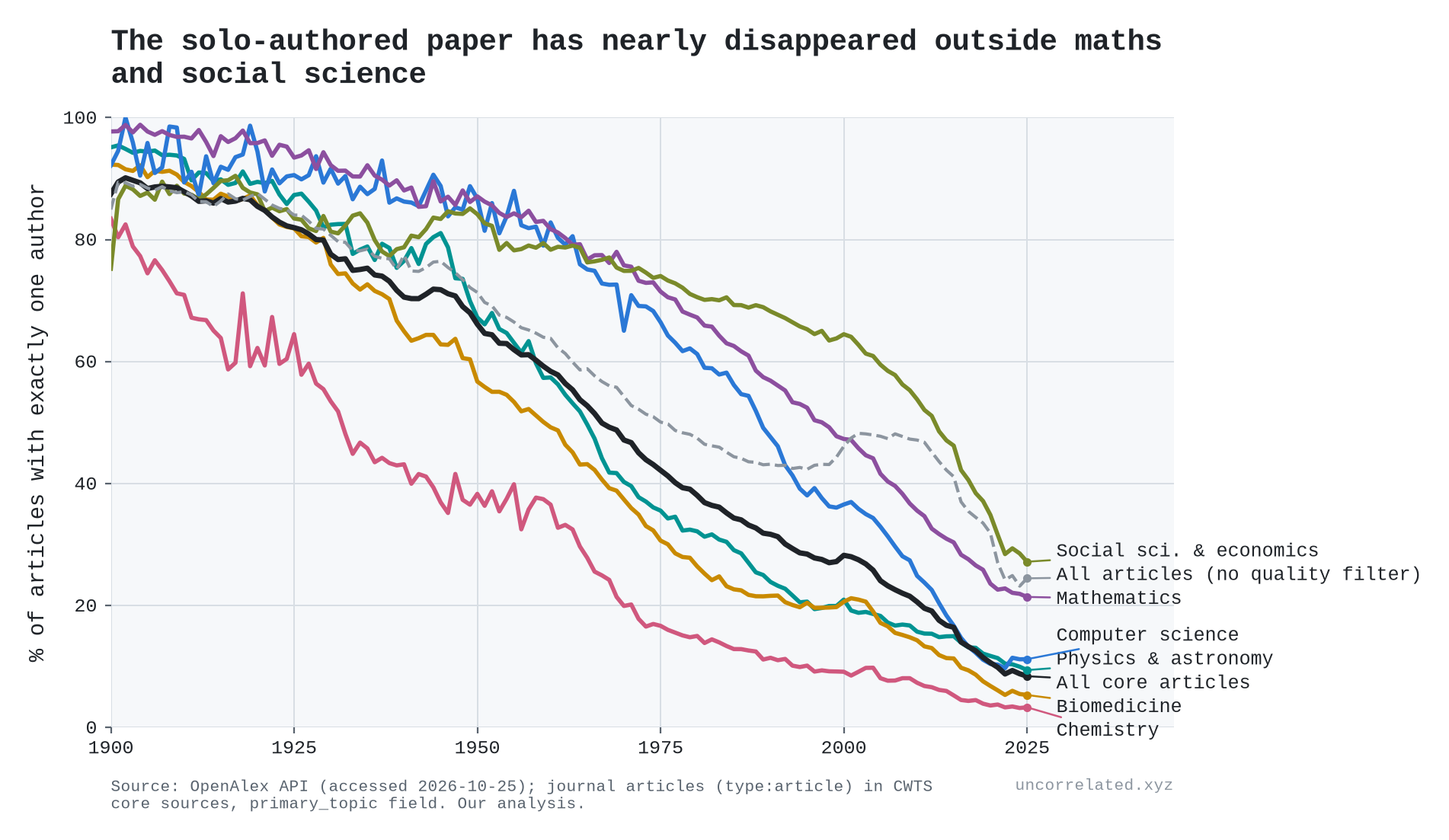
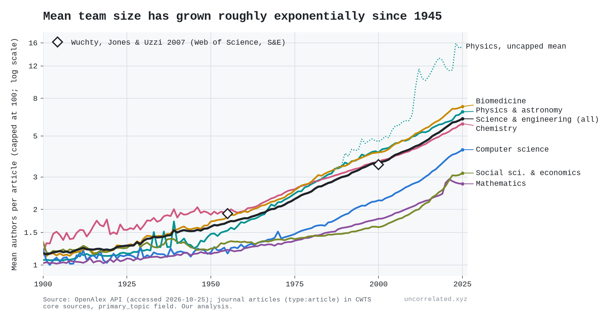
• authorship counts for every journal article in OpenAlex's core sources;
• a database of 2.3 million notable people.

Where the data cut against the thesis, I say so. In several places they do.

One terminology note. "Log-linear" can sound like a precise law. What the evidence supports is weaker and more useful: a roughly constant gain per doubling of input. Sometimes the fitted curve is a logarithm, sometimes a power law with a small exponent. Over the ranges we observe, the two are often hard to tell apart.

S1. Wright's law and learning curves

In 1936 Theodore Wright noticed that each doubling of cumulative aircraft production cut unit costs by a constant fraction, partly through better tooling (Wright, 1936, p. 124). "Wright's law" has since become the best simple predictor of technology costs. Nagy et al. tested it against Moore's law on 62 technologies and found that "Wright's law produces the best forecasts, but Moore's law is not far behind" (Nagy et al., 2013). Reviews of the wider literature find typical rates a little below our 24% median: the progress ratios in 108 factory studies cluster around 80%, a cost decline of about 20% per doubling (Dutton & Thomas, 1984, p. 238), and energy and manufacturing technologies average 16–19% (McDonald & Schrattenholzer, 2001, p. 256; Weiss et al., 2010, pp. 415–417). Solar modules sit at 20–23% (Rubin et al., 2015, p. 201; Samadi, 2018). But the spread is wide. Published estimates for solar alone run from 10% to 47%, and for onshore wind from −11% to 32% (Rubin et al., 2015, p. 201). Shipyards building an identical Liberty ship learned at anywhere from 7% to 25% per doubling (Thompson, 2012, p. 210). And in product-level data from Indian manufacturing, prices rise with cumulative output in quite a few products (Dosi et al., 2017).

Wright's law is the thesis in its cleanest form: a constant percentage gain per doubling of cumulative input.

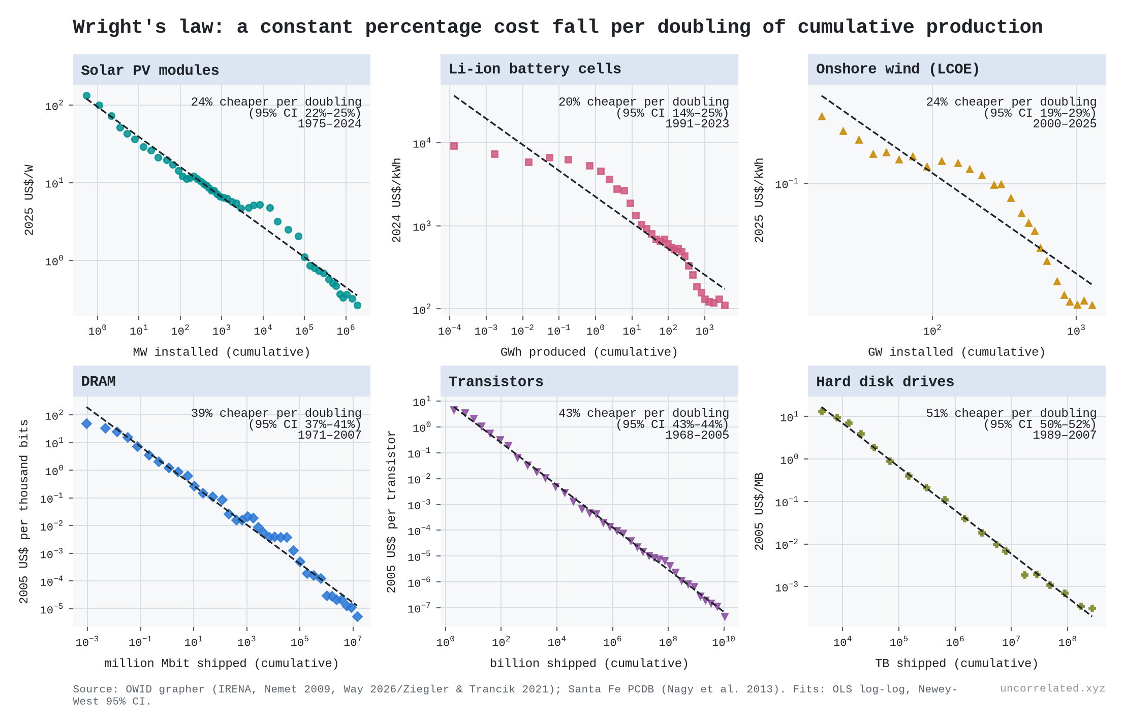
Figure 1: Cost against cumulative production on log-log axes for six technologies, with fitted learning rates (cost decline per doubling) and 95% CIs.

Our estimates (cost decline per doubling of cumulative production):

Technology	Years	Learning rate	Total cost fall
Solar PV modules	1975–2024	23.5%	499×
Lithium-ion cells	1991–2023	19.5%	83×
Onshore wind (LCOE)	2000–25	24.1%	5.6×
DRAM	1971–2007	38.6%	—
Transistors	1968–2005	43.3%	—
Hard disk drives	1989–2007	50.8%	—

Across 84 technologies in the Santa Fe Performance Curve Database, the median learning rate is 24%. Our refits reproduce Nagy et al.'s published exponents almost exactly (r = 0.9996 across 62 matched series).

Two things follow.

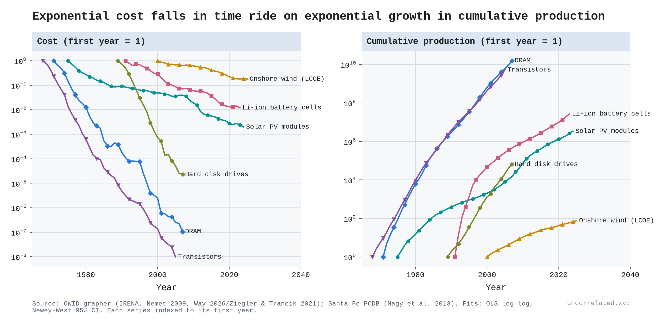
First, exponential cost declines in calendar time need exponential growth in production. The annual rate of cost decline equals the Wright exponent multiplied by the growth rate of cumulative production. For four of our six series the match is almost exact. Batteries (0.142 observed vs 0.124 implied) and wind (0.071 vs 0.067) are looser. The three closest:

Technology	Observed annual cost decline	Exponent × production growth
Solar	0.109	0.110
Transistors	0.485	0.485
Hard disks	0.650	0.651

Nagy et al. credit this point to Sahal: "A combination of an exponential decrease in cost and an exponential increase in production would make Moore's law and Wright's law indistinguishable" (Nagy et al., 2013, p. 1).

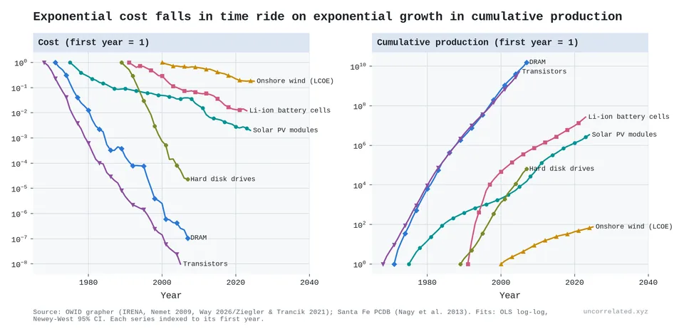
Figure 2: The same series against calendar time. Costs fall exponentially (left) because cumulative production rises exponentially (right).

Second, this is where the feedback loop comes in. Cheaper solar panels mean more solar panels get installed. That doubles cumulative production faster, which makes them cheaper still. That is why costs fell 499-fold. But the loop does not repeal diminishing returns. It hides them, by supplying the exponential input the law demands. Way et al. note that solar, wind and batteries have improved "at a rate near 10% per year" for decades (Way et al., 2022, p. 2), and this is the reason.

The constant learning rate is an approximation. Solar, battery and wind curves have steepened over the last 15 years, to 33–43% per doubling. And some technologies learn backwards: the nuclear electricity series in the Santa Fe database shows costs rising with deployment.

Fifteen technologies side by side

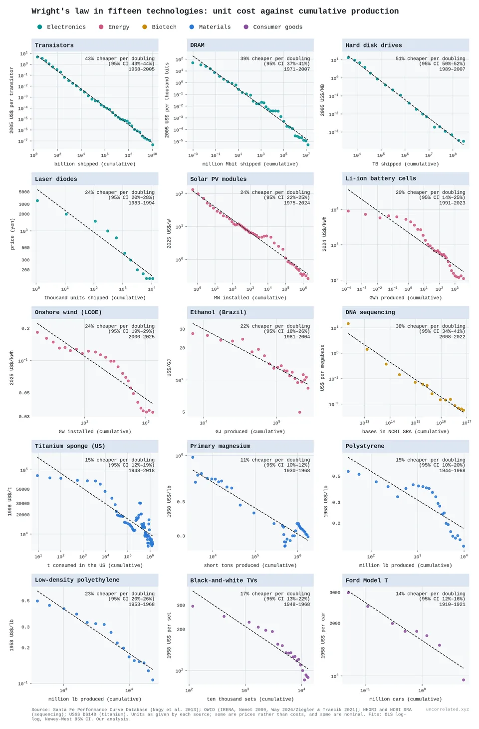
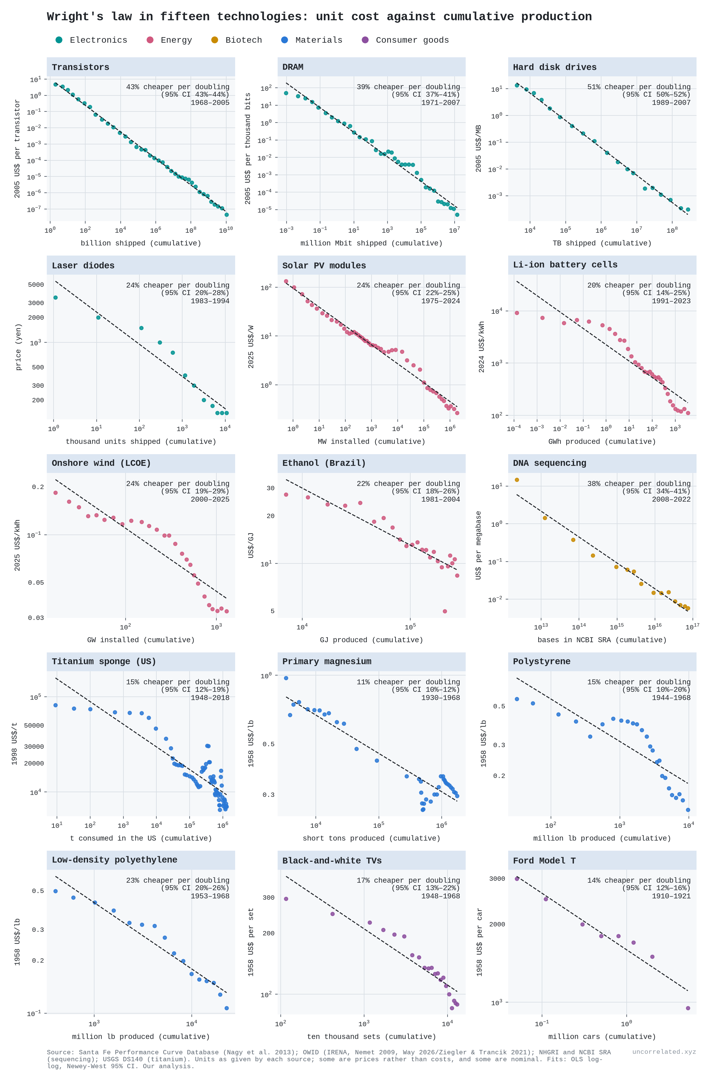
Figure 3: Unit cost against cumulative production for fifteen technologies, each in its own units, with fitted learning rates and 95% CIs. Some series are prices, not costs, and some are nominal, as in each source. Sources: Santa Fe Performance Curve Database; Our World in Data; NHGRI and NCBI; US Geological Survey. Our analysis.

The electronics and solar series sit almost exactly on their lines. Others bend. Battery and wind curves steepen late, polystyrene and magnesium start flat and then drop, and the Ford Model T has only eight points.

Titanium shows how much a learning rate can depend on the window. The Santa Fe database's titanium sponge series, 1951–68, gives 23% per doubling (Nagy et al., 2013). On the US Geological Survey's price and consumption series, which runs to 2018, the rate is 15% (95% CI 12–19%, over 17 doublings), or 19% counted from 1951. The curve is not steady either: the price was flat until 1953, fell steeply to 1972, and has since moved mostly with swings in demand. The series is a US list price for sponge alone, so it leaves out later processing and production in other countries [our analysis of USGS Data Series 140].

What is actually being accumulated?

Wright's law counts units built. But the people who study factories closely find that the units are mostly a carrier for something else.

Arrow, who made learning by doing famous, defined it as problem-solving: "Learning can only take place through the attempt to solve a problem." He added that repeating "essentially the same problem is subject to sharply diminishing returns" (Arrow, 1962, p. 155). He measured experience by new machines, not by output, because each one brings "continually new stimuli" (Arrow, 1962, p. 157).

What the inside view shows:

• Defects, found and fixed. In one car plant, defects per car and hours per car both fell about 70% in the first eight weeks of a new model. Defects fell 19% per doubling of output, and the gains tracked production, not the calendar. Teams wrote problems on whiteboards, engineers fixed them, and the knowledge ended up in the plant, not in the workers (Levitt et al., 2013, pp. 645, 656–657, 674).
• Engineering experiments. In chip fabs, yield gains are "the result of engineering experiments and analysis of production data", not of volume alone (Hatch & Mowery, 1998, p. 1463).
• Cheaper trials, more trials. At BMW a simulated crash cost about $5,000, against $150,000–600,000 for a prototype. One project ran 91 virtual crashes and improved crashworthiness by about 30% (Thomke, 1998, pp. 66–69). At Bing, the top 2% of tested ideas produced 75% of the gains, and giving each test more data helped little (Azevedo et al., 2020).

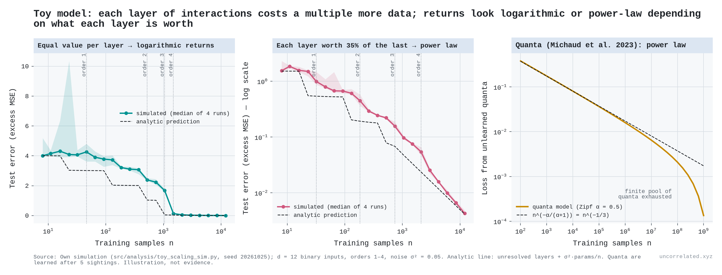
Why should that give equal steps per doubling? Think of faults on a production line. The first hundred units reveal the common ones. The next thousand reveal rarer ones. A fault that shows up once in a million units takes about a million units to find. If each layer of rarer problems is worth about as much as the last, but takes many times more attempts to uncover, every doubling buys about the same gain.

The theory behind Wright's law says the same thing. If each attempt is a random draw from the possible ways of doing a job, and the best found so far is kept, cost falls as a power of the number of draws, which is Wright's law (Muth, 1986, pp. 954–957). In design models, the exponent is set by how hard each component is to improve and how interlinked the components are. The authors note that cumulative production is only "the most commonly used proxy" for the number of attempts (McNerney et al., 2011, p. 9012).

But a lot of what the curve credits to experience is not learning at all:

• Scale. In solar, bigger plants account for 43% of the 1980–2001 module cost decline. Factors that Nemet attributes to routine production learning account for under a tenth (our grouping of Nemet, 2006, Table 3). Government and university programmes produced 10 of the 16 breakthroughs in cell efficiency while making almost none of the panels (Nemet, 2006, pp. 3225–3227). A later decomposition finds R&D the largest cause, with scale approaching it after 2001 (Kavlak et al., 2018).
• Capital. In the Liberty-ship yards, capital deepening accounts for more than half the rise in output per worker (Thompson, 2012, p. 219, summarising Thompson 2001).
• Incentives. In one chemicals firm, the steepest curves belonged to products that got process R&D, and that R&D was "not, however, generally motivated or informed, by production experience" (Sinclair et al., 2000, p. 28).
• Forgetting. Experience decays: Lockheed kept about 61% of it per year on the L-1011 (Benkard, 2000, p. 1049).

So cumulative production is a bundle: trials in the factory, trials in the lab that a growing market pays for, and plain scale. Only the first two are learning. The data cannot cleanly separate them, because every cumulative series trends upward together, and learning rates estimated from such series tend to be biased upward (Thompson, 2012; Nordhaus, 2014).

For the thesis, this matters in one direction. If the true input is informative trials, and repetition yields less each time, a log-shaped return is what we should expect. Cheap trials (simulation, A/B tests, faster sequencing) raise progress by raising the count of trials, not by changing the shape of the curve.

A counterexample: DNA sequencing

Sequencing is the standard objection. Its costs fell much faster than Moore's law.

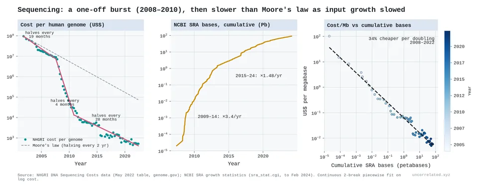
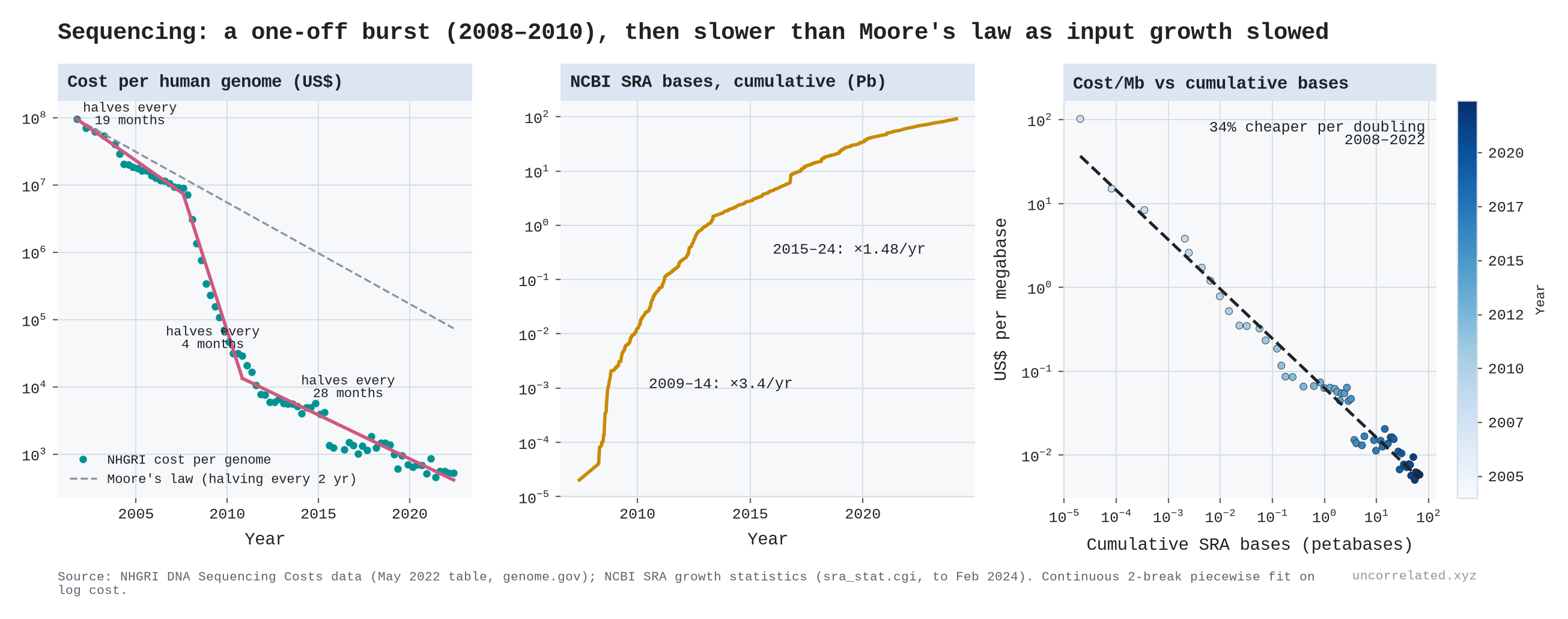
Figure 4: Cost per genome against a Moore's-law line (left), cumulative bases in NCBI's Sequence Read Archive (middle), and cost per megabase against cumulative bases sequenced (right).

The data show a burst, not a faster law:

• Before: cost per genome halved every 19 months (2001–07), roughly Moore's pace.
• The burst: with next-generation sequencing it halved every 4 months (2007–10).
• After: it slowed to a halving every 28 months, slower than Moore.
• Input: cumulative bases sequenced grew 3.4× a year in 2009–14 and 1.5× a year in 2015–24.
• One curve: a single Wright curve, a 34% cost decline per doubling of cumulative bases sequenced, fits all of 2008–22.

A paradigm shift opened a new field of low-hanging fruit. Costs collapsed while it was harvested, then progress returned to a constant gain per doubling. I would describe the overall pattern as a sawtooth around a log trend. New tools briefly raise research productivity, and then the usual diminishing returns resume.

Is the input units or calendar time?

When production grows at a steady exponential rate, cumulative units and calendar time are nearly the same variable, which is Sahal's point above. I set out a test before running it: fit log cost against log cumulative units and against the year, then compare the scatter around each line and how well a line fitted to the first half of the years predicts the second half.

Units gave the better fit in 9 of 14 comparisons. They won on both criteria for solar, transistors, hard disks and DNA sequencing. Time won on both for batteries and onshore wind, and DRAM was split [our analysis]. Sequencing shows the difference most clearly. Its cost fell 73% a year in 2008–12, 34% in 2013–17 and 20% in 2018–22, but 45%, 42% and 42% per doubling of the bases sequenced. The pace per year slowed because bases doubled less often [our analysis].

The older literature reaches the same mixed verdict. Regressions of cost on cumulative output and on time usually fit about equally well when run separately, and the usual way of separating them can wrongly favour output when errors persist from year to year (Thompson, 2012, pp. 214–215).

Is the input trials or dollars?

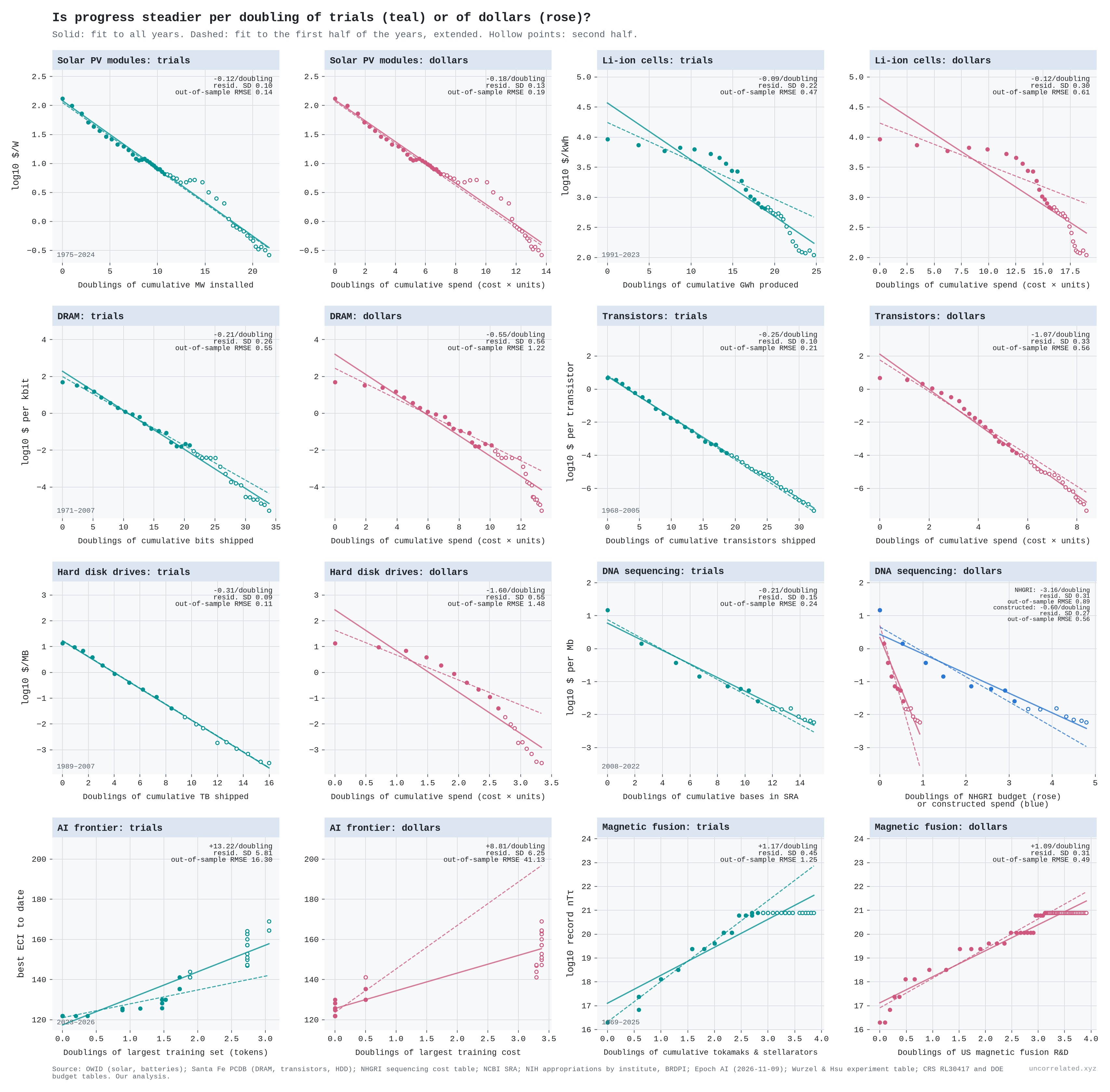
If progress comes from what we learn, the real input may be the number of informative trials: bases sequenced, tokens trained on, prototypes tested. Units built are only a rough stand-in, for the reasons above. Money only buys them, and the price of a trial keeps changing. If so, progress should be steadier per doubling of trials than per doubling of dollars. I set the test out before fitting anything. For each case I fitted the output against the logarithm of each input, then compared three things: how tightly the points sit around each line, how stable the gain per doubling is across three periods, and how well a line fitted to the first half of the years predicts the second half.

Trials gave the steadier line in eight of nine cases (Figure 5). On average the scatter around the dollar line was 1.8 times larger, and its errors on the second half were twice as large [our analysis]. But most of that win is less independent than it looks.

• Learning curves. For solar, batteries, DRAM, transistors and hard disks, the only dollar series is the money spent on the units themselves: unit cost times units. Where that spending kept growing, the dollar line is nearly as good. Spending on solar modules grew 18% a year, from $54 million in 1976 to about $120 billion in 2024, even as each watt got 500 times cheaper. Where spending stopped growing, the dollar line fails. In the Santa Fe data, spending on hard disks fell about 2% a year while their cost kept falling, and the scatter around the dollar line is six times larger. Because these dollar series are built from the unit counts, and units bundle trials with scale, these cases cannot test the idea on their own.
• Sequencing. Cost per megabase fell about 2,500-fold over 2008–22. Per doubling of bases sequenced it fell by a steady 42% in each five-year period (on annual data; the 34% above comes from quarterly data). NHGRI's budget was flat in real terms, so its cumulative total did not quite double, and the gain per doubling of its money swung from 6.6 to 1.8 orders of magnitude. NHGRI is only a small part of what the world spends on sequencing, though.
• AI. Neither input is steady. Both the largest training set and the largest training budget rose in steps. The budget did not move for the last year of the sample while the capability index rose 19 points.
• Magnetic fusion is the one case where dollars won. Since 1997 the number of tokamaks and stellarators in Wurzel and Hsu's table has doubled, from 14 to 29, with no new record, while US spending rose 66%. One reading is that, like extra robot demonstrations in the same homes, more machines of the same size were not informative trials for the record. But that is an explanation after the fact; counted plainly, this case goes against the idea. Over 1969–98, while records were still being set, the machine count won all three tests: each doubling of machines bought about 1.7 orders of magnitude of triple product (95% CI 1.6–1.8) [our analysis].

The pattern is simple: the steadier input is whichever one kept growing exponentially. Trials usually did, because each one got cheaper. Dollars did only when falling prices drew in more spending, which is the feedback loop above. That fits the reading that the law is about trials and money is the means of buying them. It is not a clean test. In most cases the dollar figures are built from the trial counts, and of the three cases with independent dollar series, one favours trials, one is a tie and one favours dollars.

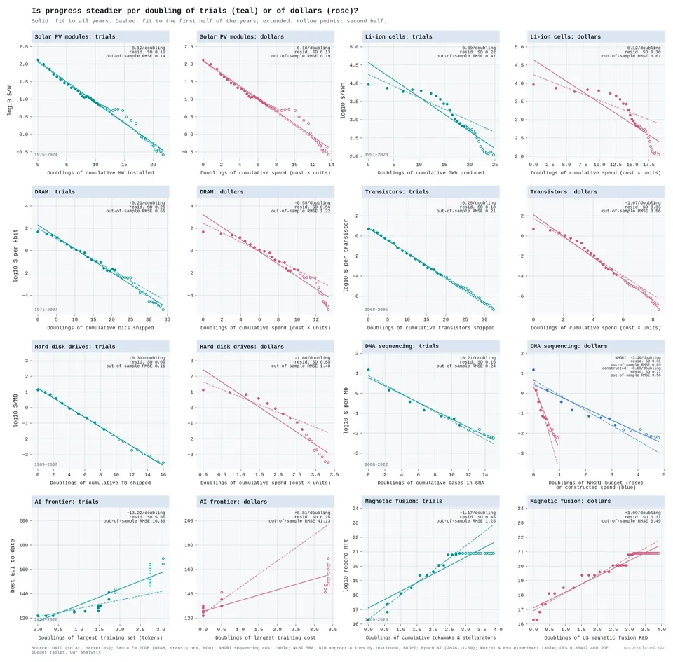
Figure 5: Output against doublings of cumulative trials (teal) and of cumulative dollars (rose), with the same y-axis for each pair. Solid lines are fits to all years. Dashed lines are fitted to the first half of the years and extended. Hollow points are the second half. Trials: units produced; bases in NCBI's Sequence Read Archive; the largest training set to date; tokamaks and stellarators in Wurzel and Hsu's table. Dollars: unit cost times units produced; NHGRI appropriations (rose) and bases times cost (blue); the largest training cost to date; US magnetic fusion R&D. Sources: OWID; Santa Fe Performance Curve Database; NHGRI; NCBI; NIH appropriations by institute; Epoch AI; Wurzel & Hsu; CRS RL30417; DOE budget tables. Our analysis.

S2. Ideas are getting harder to find

The anchor is Bloom, Jones, Van Reenen and Webb's "Are Ideas Getting Harder to Find?" (Bloom et al., 2020). They define research productivity as the growth rate of ideas divided by the number of effective researchers, then measure it everywhere they can.

Their aggregate measure of "ideas" is total factor productivity (TFP) growth. TFP is a residual: the part of economic growth not explained by more capital and labour. It is noisy, and it is sensitive to how capital and quality are measured. I don't want the argument to rest on it. So I treat the aggregate TFP result as one line of evidence among several, and put more weight on outcomes measured physically: transistor density, crop yields, cost per unit of a technology, model loss, and genetic discoveries.

Their replication files are public, so I re-ran their aggregate, Moore's-law and crop-yield calculations from the original data. Everything matches to rounding:

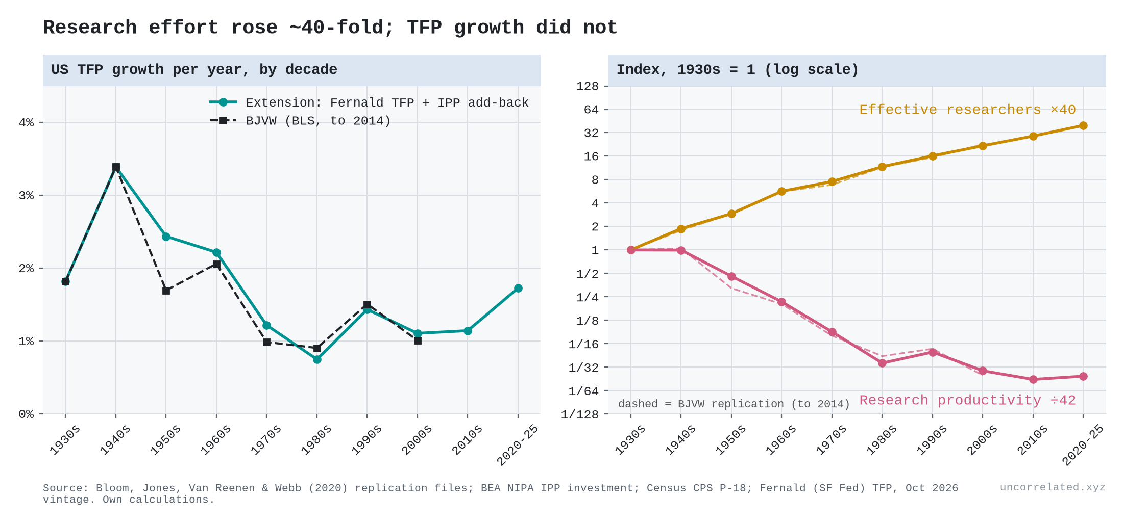
• Aggregate US: effective research effort rose 22.7-fold (4.3% a year) from the 1930s to the 2000s, and research productivity fell 40.9-fold (−5.1% a year, half-life about 13.5 years). The paper reports 23-fold and 41-fold (Bloom et al., 2020, p. 1110).
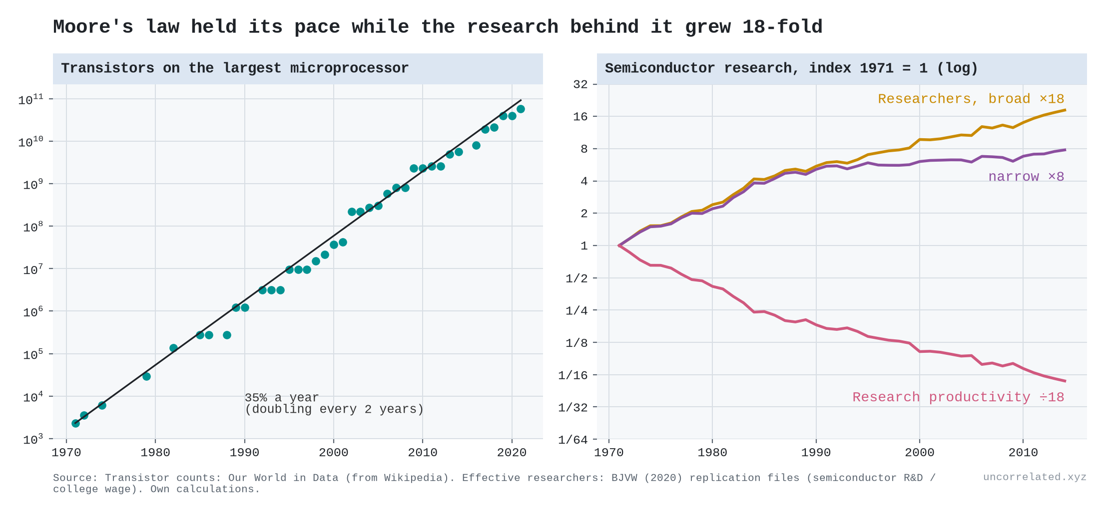
• Moore's law: keeping chip density doubling roughly every two years took 18 times more semiconductor research effort over 1971–2014 than at the start. Research productivity fell 6.8% a year (Bloom et al., 2020, Table 1).
• Crops: counting only research on seed efficiency, research productivity for corn, soybeans, cotton and wheat fell by factors of 52, 19, 4 and 12 (Bloom et al., 2020, Table 2). Including crop-protection research, the falls are smaller, and for cotton research productivity rose.

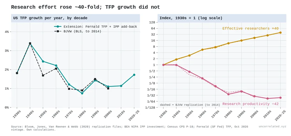
Figure 6: Left: US TFP growth per year by decade, from Bloom et al.'s data (dashed, to 2014) and our extension with Fernald's TFP series (solid, to 2025). Right: effective researchers rose about 40-fold since the 1930s while research productivity fell about 42-fold. Log scale.

Then I extended the series to 2025 using current BEA, Census and San Francisco Fed data. Over the whole period the picture survives: effort is up about 40-fold and research productivity down about 42-fold, falling 4.2% a year.

The extension also shows something the original paper could not: since the 1980s, the decline has nearly stopped. From the 1980s to 2020–25, research productivity fell only about 1% a year between endpoints, and a fitted trend over the same decades (−1.7% a year) has a confidence interval that includes zero. TFP growth recovered from 0.75% a year in the 1980s to 1.7% in 2020–25, while research effort grew 3.2% a year. The recent window is short and includes the pandemic, so I wouldn't lean on it. But anyone telling a clean "ideas keep getting harder" story should know it is there.

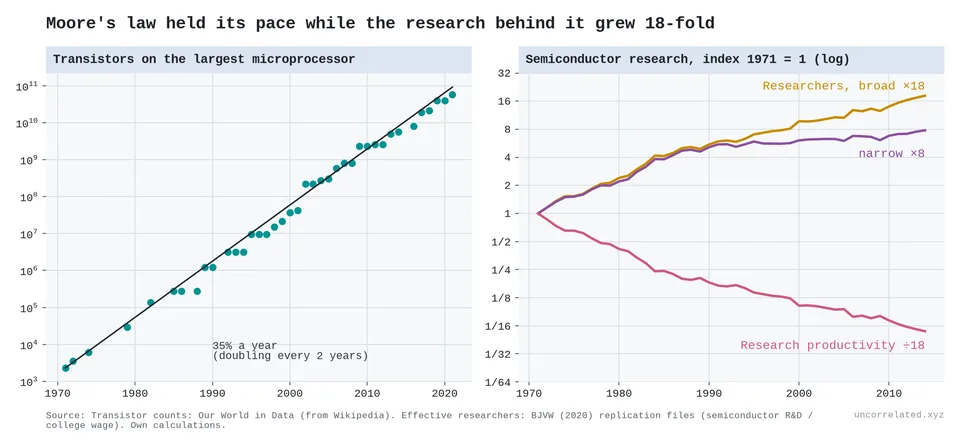
Figure 7: Frontier transistor counts grew at about 35% a year (our estimate: 34.95%, 1971–2021). Semiconductor research effort rose 8–18-fold to sustain that, so research productivity fell about 18-fold.

One more check on Moore's law. Bloom et al. assume a constant 35% annual growth in transistor density. Our fit to frontier chips gives 32% (1971–90), 39% (1990–2010) and 31% (2010–21). The rate did move between periods: both the 1990–2010 speed-up and the post-2010 slowdown are statistically clear. But it stayed within a few points of 35% throughout, and the post-2010 rate is not significantly below 35%. The treadmill ran at a roughly constant speed; it just took ever more people to keep it running.

What shape is the curve? Functional forms

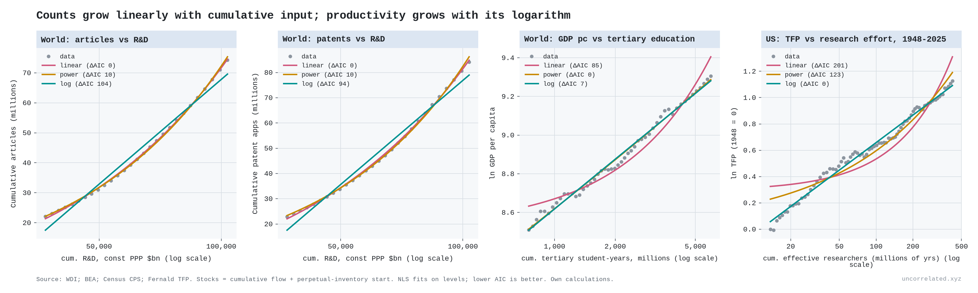
"Diminishing returns" can mean several different things, so I fitted three functional forms to cumulative output against cumulative input: linear, power law and logarithmic.

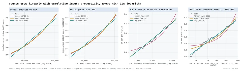
Figure 8: Counts grow linearly with cumulative input; productivity grows with its logarithm. Left two panels: world cumulative articles and patents against cumulative R&D spending, where linear wins and log loses badly. Right two panels: world GDP per capita against cumulative tertiary education, where the power form fits better (ΔAIC 7) though the log form is close in shape, and US TFP against cumulative effective researchers (1948–2025), where the log form wins clearly.

The answer depends entirely on what you count as output.

• Counts scale with input. World cumulative articles and patents grow linearly or slightly faster with cumulative R&D spending. The elasticities are 1.2 and 1.3, and the log form is rejected by a wide margin. World articles per researcher actually rose 1.7% a year over 2000–2020. Exponential input produces an exponentially growing literature, which is what the thesis expects. The diminishing returns are not in how much gets produced but in how far each unit moves the frontier.
• Growth is logarithmic. For US TFP against cumulative effective researchers, 1948–2025, the log form beats the power form by 123 AIC points and the linear form by 201. It also forecasts out of sample far better: 3.5% error against 21% and 52%. Each doubling of cumulative research buys about 0.21 log points of TFP (95% CI 0.20–0.22). The log form still wins when the assumed starting knowledge stock is scaled anywhere from a quarter to four times our baseline; the gain per doubling then ranges from 0.17 to 0.31.
• World GDP sits in between. Against cumulative R&D the power and log forms fit about equally well; against cumulative tertiary education the power form is clearly ahead (ΔAIC 7); a power law with an exponent of about 0.05 on log GDP is practically a logarithm. Only the 78-year US series has enough curvature to separate the two.

Put together, the two results resolve an old argument. Optimists point to ever more papers and patents. Pessimists point to flat productivity growth. Both are right. We produce more and more units of knowledge, but each unit moves the frontier less. Rescher's version is "scientific knowledge does not correlate with the brute volume of scientific information, but only with its logarithm" (Rescher, 1999, p. 43).

The world: exponential inputs, flat growth

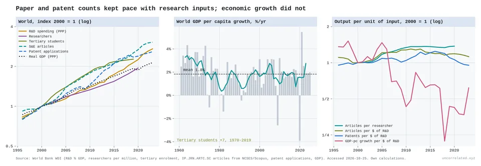
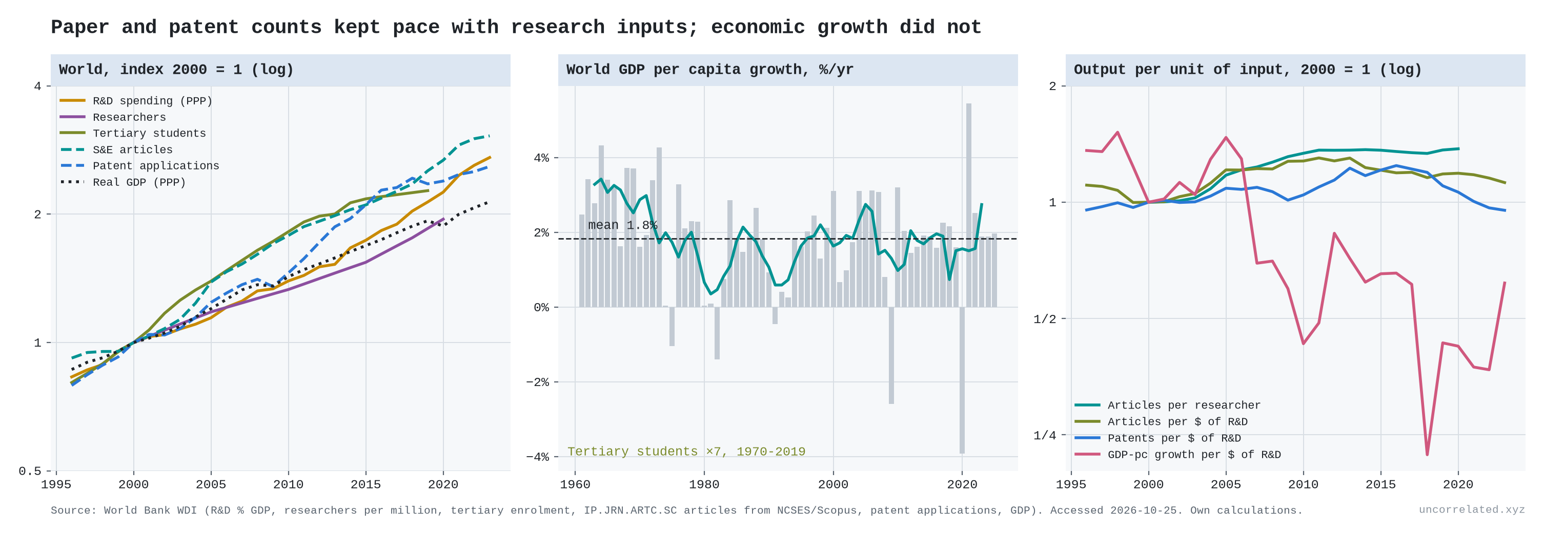
Figure 9: World input and output indices (left); world GDP-per-capita growth, 1961–2024, flat at about 1.8% a year (middle); output per unit of input (right). Papers and patents per dollar are flat or rising, while GDP growth per dollar of R&D falls about 5.7% a year.

At world scale:

• Inputs: R&D spending (constant PPP) grew 4.2% a year over 1996–2023, from $1.3 trillion to $4.4 trillion, doubling every 16 years. Researchers grew 3.1% a year (2000–2020). Tertiary enrolment rose from 32 million in 1970 to 228 million in 2019.
• Growth: world real GDP-per-capita growth averaged 1.84% a year from 1961 to 2024. Its trend was −0.15 percentage points per decade, which is essentially flat.
• Productivity: GDP growth per R&D dollar fell 5.7% a year. That is close to Bloom et al.'s US estimate of 5.1%, from completely different data, although the world series is noisy.

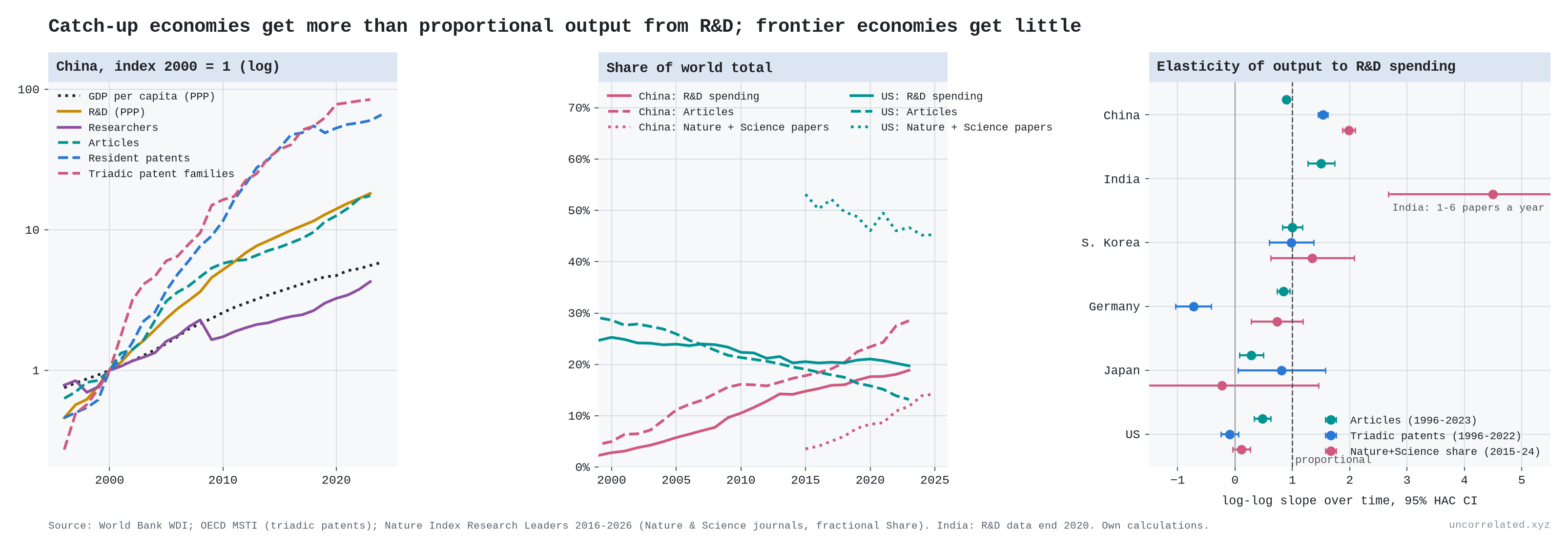
A caveat on composition. China accounts for about 90% of the growth in world resident patents since 2000 and about 40% of the growth in articles; its share of world resident patents rose from about 3% in 2000 to 60% in 2023. Aggregates hide a lot, and I return to China below.

S3. The cases in the table, one by one

This section covers the rows of the main post's table that are not treated elsewhere. Solar, the Santa Fe technologies, DNA sequencing and the fusion machine count are in S1. Genetic prediction is in S4. Language-model error, AI capability and robots are in S5. Where this section says "worse than logarithmic", the table says "faster than log (diminishing returns)"; "better than logarithmic" is the table's "closer to linear (accelerating returns)".

TFP is a residual, so I also ran the same tests on outputs measured physically, each against its own R&D input. For each one I asked two questions. Does each doubling of cumulative R&D buy the same gain, decade after decade? And does the curve bend down (worse than logarithmic) or up (better)? None of these output series comes from Bloom et al.

Crop yields

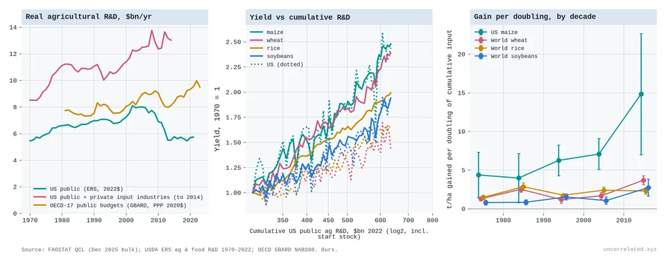
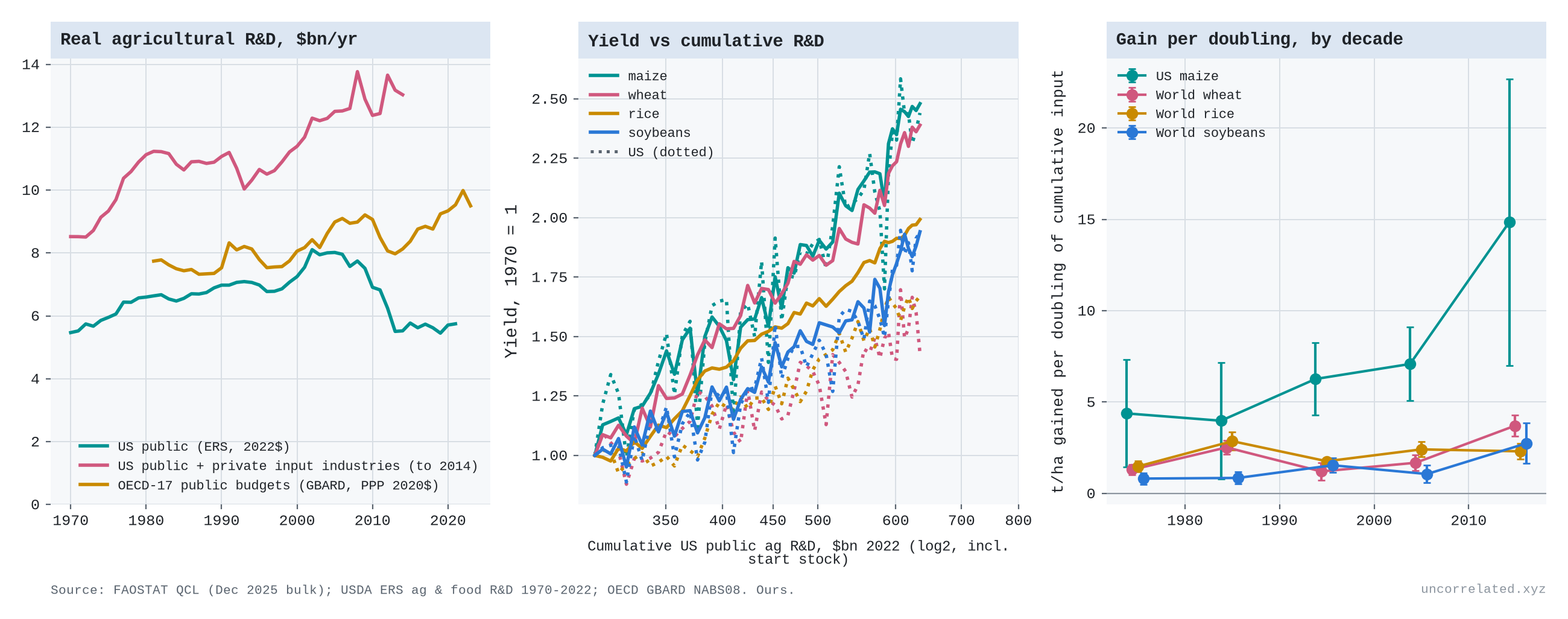
Figure 10: Left: real agricultural R&D (US public, US public plus private input industries to 2014, OECD-17 public budgets). Middle: crop yields (1970 = 1) against cumulative US public agricultural R&D, log scale; solid lines world, dotted US. Right: tonnes per hectare gained per doubling of cumulative input, by decade, with 95% CIs. Sources: FAOSTAT; USDA ERS; OECD GBARD.

• Crop yields do better than logarithmic against public R&D.
  • Real US public agricultural R&D was flat from 1970 to 2021, and has fallen since its 2002 peak.
  • Yields kept rising by about the same tonnes per hectare every year: US maize by 0.11 t/ha a year in 1961–90 and 0.12 in 1990–2024.
  • So each doubling of cumulative public R&D bought more over time: 4.4 t/ha of US maize in the 1970s, 14.9 in the 2010s.
  • The logarithmic shape only returns once private R&D by agricultural input companies (seeds, chemicals, machinery) is included. That input grew from $3.1 billion to $7.5 billion a year between 1970 and 2014. With it, world wheat and rice are close to log-linear. US maize still edges up (3.2, 3.0, 5.3 and 5.8 t/ha per doubling from the 1970s to the 2000s), though the bend is no longer statistically significant.
  • The result also depends on an assumption about the starting stock of R&D, because when spending is flat the number of "doublings" is small.
  • Measured as percentage growth, world wheat and rice yields are slowing.

US life expectancy

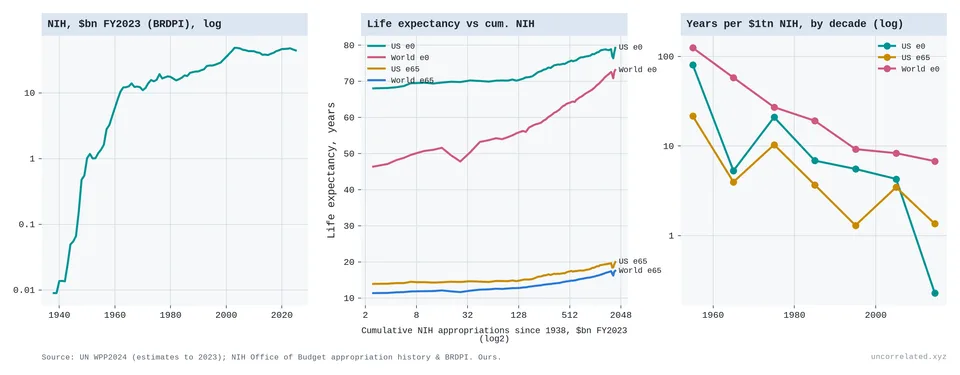
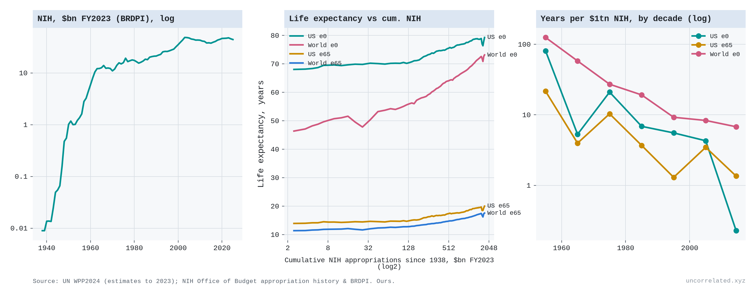
Figure 11: Left: real NIH appropriations (FY2023 dollars, log scale). Middle: life expectancy at birth and at 65, US and world, against cumulative NIH spending since 1938 (log scale). Right: years of life expectancy gained per $1 trillion of real NIH spending, by decade (log scale). Sources: UN World Population Prospects 2024; NIH Office of Budget.

• US life expectancy fits the thesis, then stalls.
  • Against cumulative NIH spending, 1970–2019, the logarithmic form fits best, at about 2.4 years of life expectancy per doubling. It held at about 2–3 years per doubling through the 2000s.
  • Then the 2010s bought almost nothing: 0.2 years per doubling.
  • Measured per dollar, years gained per $1 trillion of real NIH spending fell from 21 in the 1970s to 0.23 in the 2010s, roughly a hundredfold.
  • Life expectancy is driven by far more than NIH (smoking, income, public health, opioids), so this is co-movement, not a causal estimate.

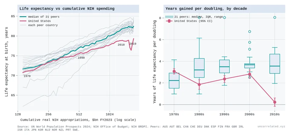
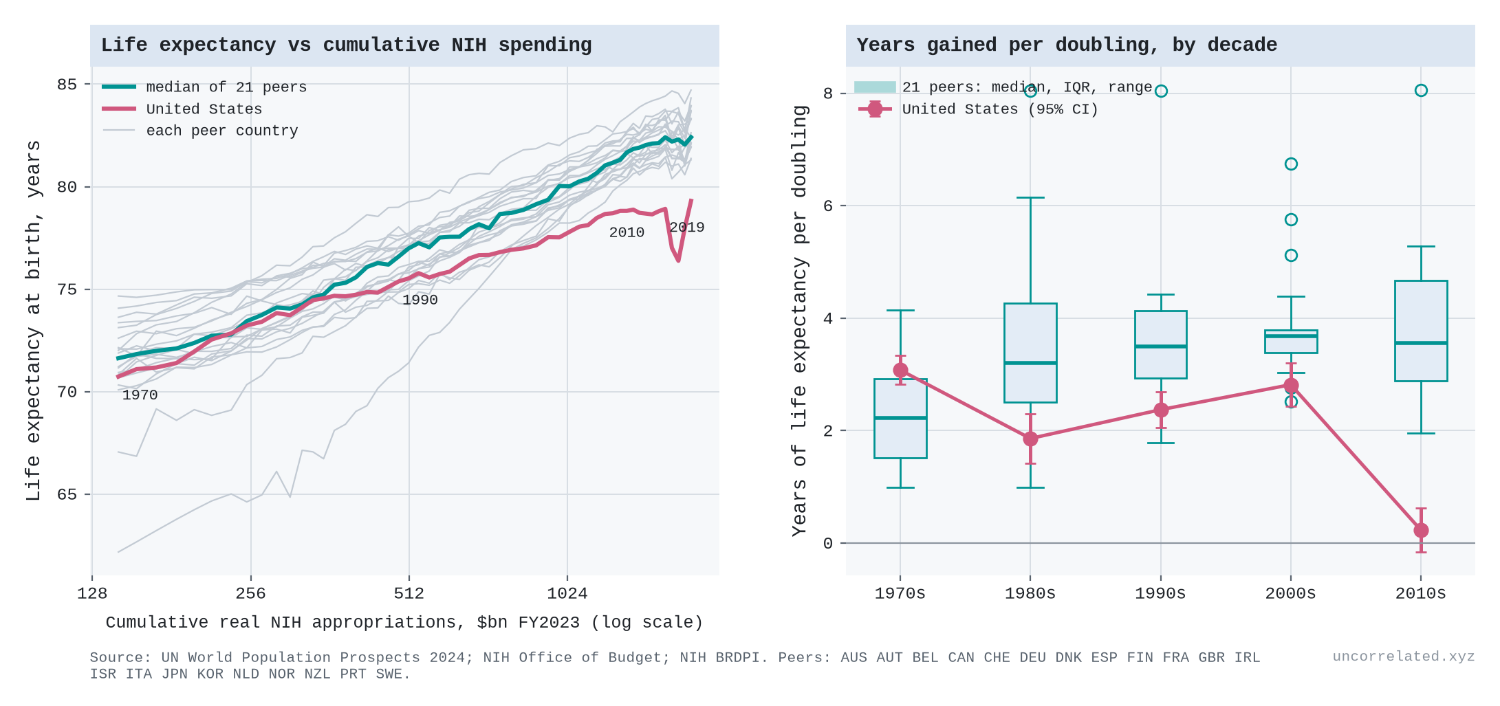
Figure 12: Left: life expectancy at birth against cumulative real NIH spending, the US and 21 high-income peers (grey; teal, their median). Right: years gained per doubling, by decade; boxes show the peers, rose the US with 95% CIs. NIH stands in for the world's biomedical knowledge stock, which it is not; the input is the same for every country. Sources: UN WPP 2024; NIH Office of Budget.

• But the stall is American, not a limit on medical knowledge. If the 2010s collapse reflected diminishing returns to biomedical research, other rich countries, which draw on the same global stock of medical knowledge, should have stalled too. They didn't.
  • Across 21 high-income peers, the median gain per doubling was 2.2, 3.2, 3.5, 3.7 and 3.6 years in the 1970s, 80s, 90s, 2000s and 2010s.
  • The US went from 3.1 to 0.2. It ranked last of the 22 in the 2010s, and every peer gained about 2 years or more per doubling in that decade.
  • Against all US biomedical R&D (NIH plus pharmaceutical industry), the peer median is close to log-linear, bending slightly down: 2.4–4.1 years per doubling in every decade.
  • Against NIH spending alone, the peers did better than log-linear: the median gain per doubling rose from 2.2 to about 3.6 years, and a power form fits best.
  • So the health case is consistent with the thesis, with the verdict depending on the input: log-linear against all US biomedical R&D, better than that against NIH alone. Either way, the US stall is a US problem, from whatever causes it, not evidence that medical progress ran into a wall.

New drugs

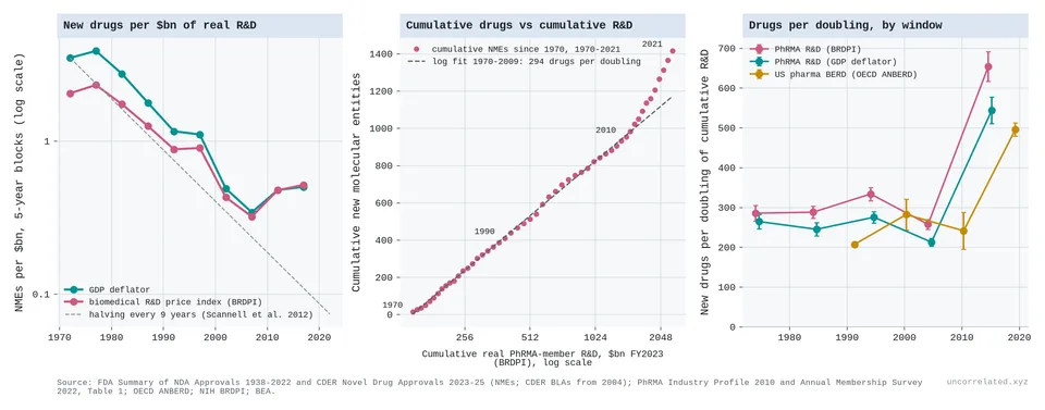
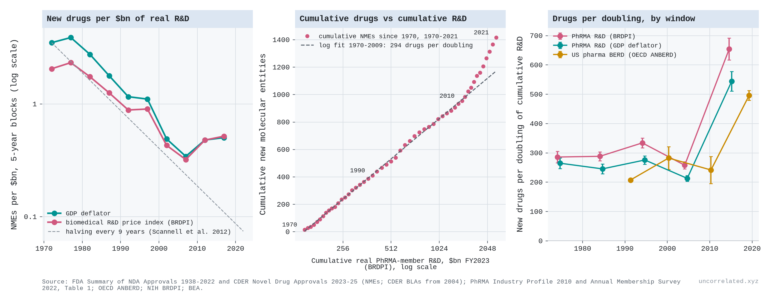
Figure 13: Left: new molecular entities approved by the FDA per $billion of real pharmaceutical R&D (PhRMA members), five-year blocks, with Scannell et al.'s nine-year halving. Middle: cumulative new drugs since 1970 against cumulative real R&D (log scale), with the 1970–2009 logarithmic fit. Right: new drugs per doubling of cumulative R&D, by decade, for three R&D series. Sources: FDA; PhRMA; OECD ANBERD; NIH BRDPI; BEA.

• New drugs: Eroom's law is the logarithmic law seen from the other side. Scannell and colleagues showed that new drugs approved per billion dollars of R&D "halved roughly every 9 years since 1950" (Scannell et al., 2012, p. 191). We reproduce that from FDA and industry data: −7.1% a year over 1970–2009 with R&D deflated by the GDP deflator, a halving every 9.8 years (12.3 years with the NIH biomedical price index).
  • But falling drugs per dollar is exactly what log-linear returns look like when spending grows exponentially. Cumulative new drugs rose by an almost constant 260–330 per doubling of cumulative real R&D, decade after decade from 1970 to 2009.
  • The logarithmic form beats power and linear forms by a wide margin (ΔAIC 45 and 73), and before 2004, when the FDA count changed to include biologics, the curve has no detectable bend.
  • New drugs behave like frontier knowledge, not like papers or patents. Each has to clear a fixed bar of being new and working.
  • Then the law broke, upwards. Since about 2010, each doubling has bought about twice as many new drugs (496–655 on the three R&D series), while R&D growth slowed. It is another better-than-logarithmic episode, like sequencing and crop yields. Approvals are counts, not value: many of the recent ones are for rare diseases and cancers.

Chips, supercomputers and GPUs

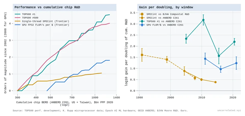
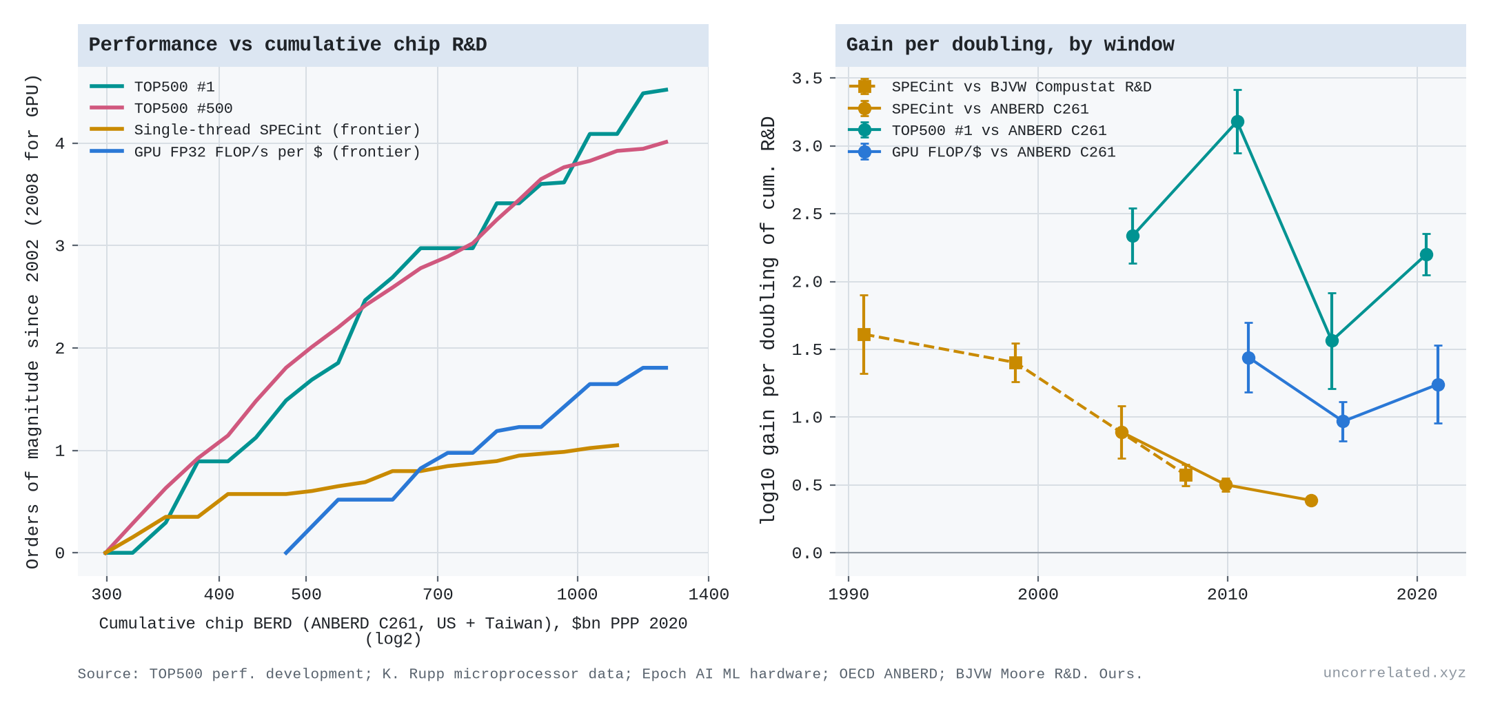
Figure 14: Left: orders of magnitude of performance gained since 2002 against cumulative semiconductor R&D (OECD ANBERD, US and Taiwan). Right: orders of magnitude gained per doubling of cumulative R&D, by window, with 95% CIs. The dashed series in the right panel uses Bloom et al.'s Compustat semiconductor R&D as the input instead. Sources: TOP500; K. Rupp microprocessor trend data; Epoch AI; OECD ANBERD; Bloom et al.

• Computing splits.
  • Single-thread processor speed does worse than logarithmic. Against OECD industry R&D, each doubling of cumulative chip R&D bought 0.89, then 0.50, then 0.39 orders of magnitude of speed, over 2002–08, 2008–13 and 2013–17. The gain per doubling more than halved.
  • Supercomputer performance and GPU price-performance are close to log-linear, bending down slightly.

Three more cases where progress is bought almost entirely with compute, and where the outputs are measured directly:

Weather forecasts

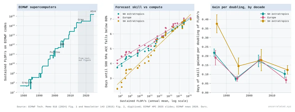
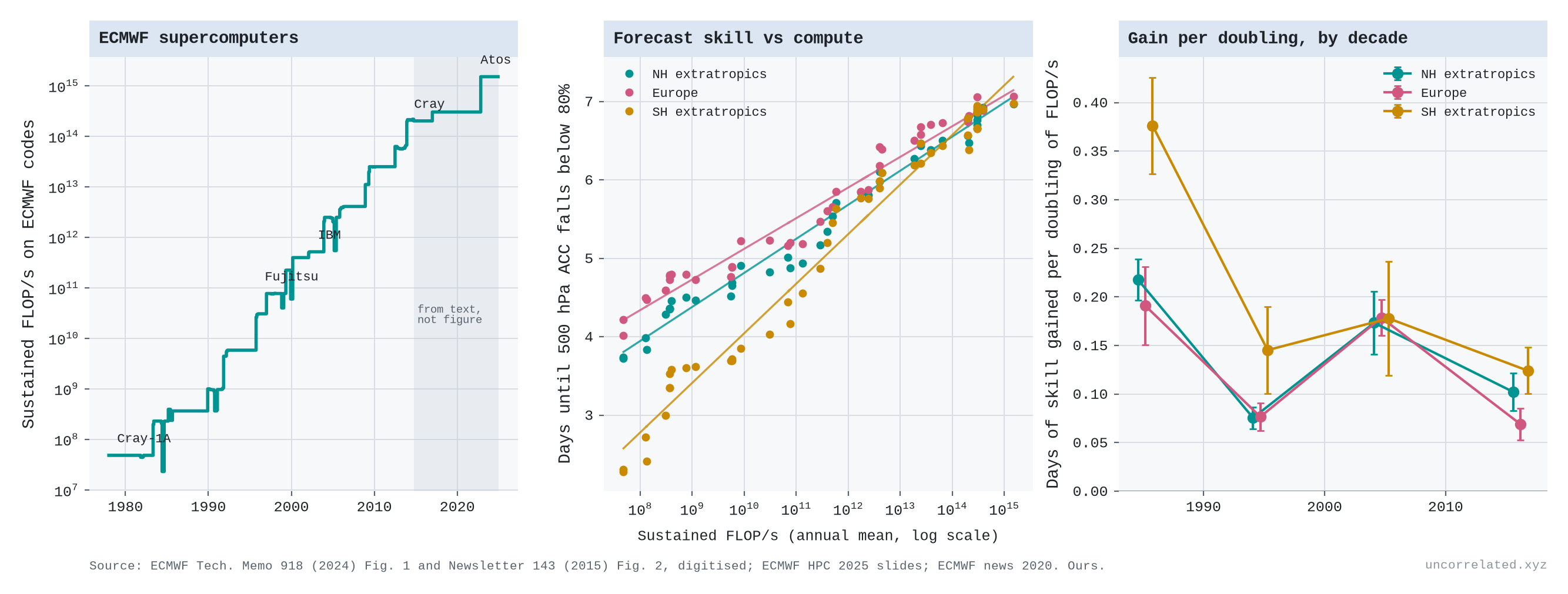
Figure 15: Left: sustained performance of ECMWF's supercomputers on its own codes. Middle: forecast skill (the lead time, in days, at which the 500 hPa anomaly correlation falls below 80%, annual means) against sustained FLOP/s, with logarithmic fits. Right: days of skill per doubling of compute, by decade. Skill and compute to 2014 are digitised from ECMWF publications; compute after 2014 is inferred from statements in ECMWF texts (shaded).

• Weather forecasts are the cleanest log-linear case we found. Between 1981 and 2023 the European Centre's sustained computing power rose by about 25 doublings, and the range of a useful Northern Hemisphere forecast grew from 3.7 to 7.0 days (Haiden et al., 2024; Hawkins & Weger, 2015).
  • That is about 0.13 days of forecast per doubling of compute, with no detectable bend over 25 doublings. The logarithmic form beats the linear one overwhelmingly and the power form slightly.
  • With a one-year lag, compute predicts Northern Hemisphere skill better than a simple time trend does; with no lag the two are about equal. For Europe and the Southern Hemisphere, compute wins at any lag. When compute growth slowed after 2014, to about a third of a doubling a year from 0.86 in the 1990s, skill gains slowed too: from 1.2 days per decade in 2000–10 to 0.5 in 2010–23. The post-2014 compute figures are inferred from statements in ECMWF's texts, not from published series.
  • Underneath the straight line is a sawtooth. Per decade, a doubling bought 0.22, 0.08, 0.17 and 0.10 days. The 1990s, the decade with the most new compute, bought the least.
  • At the 2014–23 rate of growth, one more day of forecast needs about 200 times today's compute and about 24 years.
  • A break may be coming. Machine-learning forecasts trained on past weather, including ECMWF's own AIFS and Google DeepMind's GraphCast, are now competitive with the physics model on upper-air skill (Haiden et al., 2024). They are reportedly far cheaper to run, though we did not measure that.

Mersenne primes

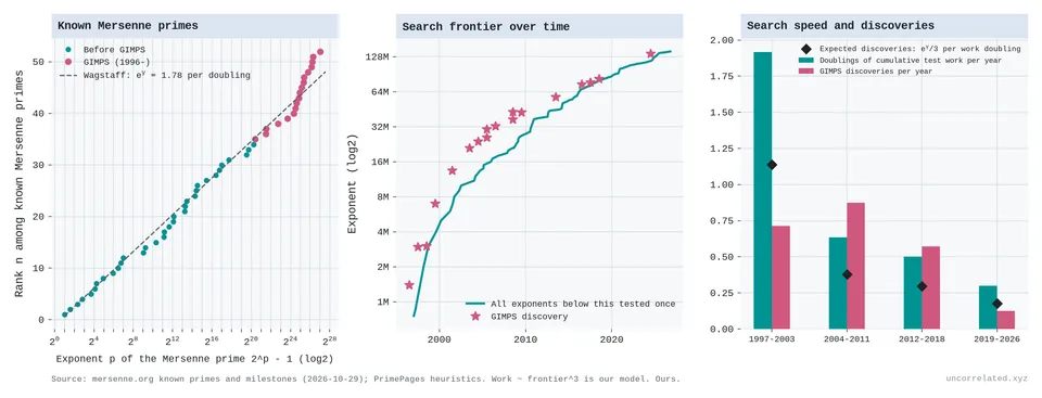
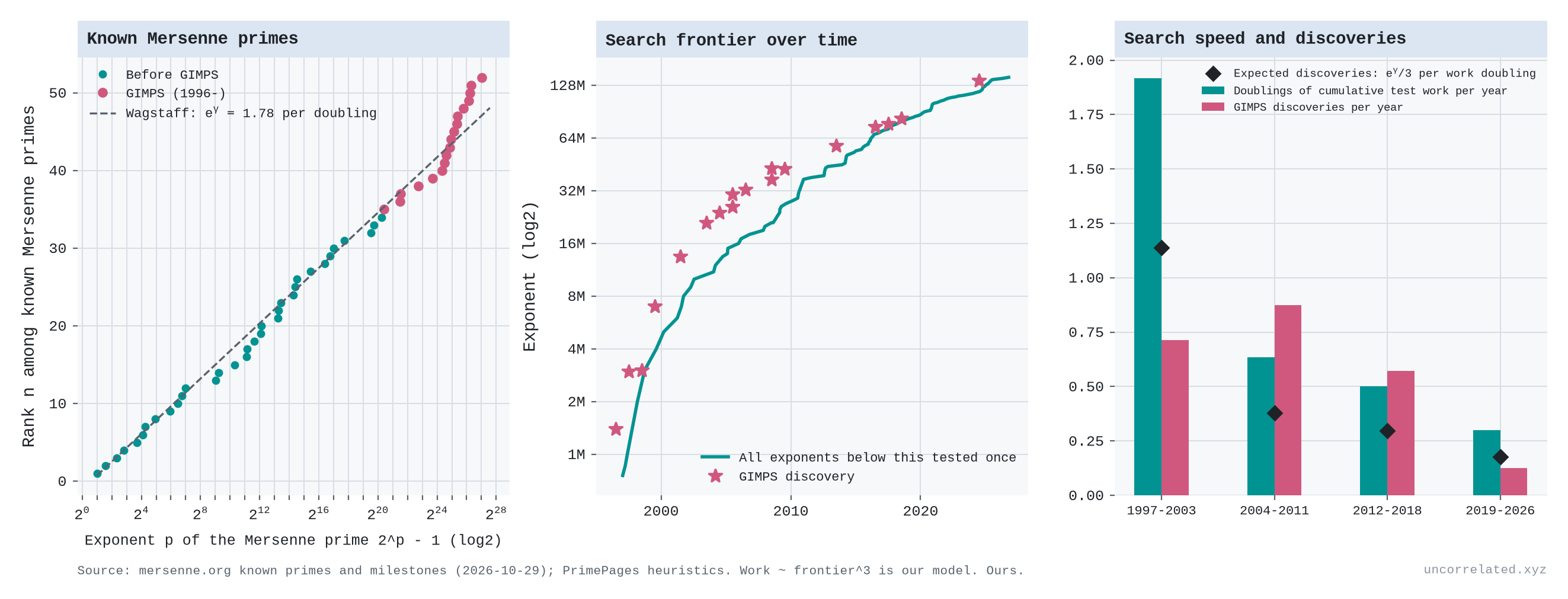
Figure 16: Left: rank of each of the 52 known Mersenne primes against its exponent (log scale), with the heuristic of e^γ ≈ 1.78 primes per doubling. Middle: the Great Internet Mersenne Prime Search's frontier (all exponents below it tested) and its discoveries. Right: doublings of cumulative test work per year and discoveries per year, with the number expected. Sources: mersenne.org; PrimePages.

• Prime hunting has a log-linear law built into the mathematics, or at least into a well-tested conjecture. Wagstaff's heuristic says the expected number of Mersenne primes with exponent between x and 2x is a constant, e^γ ≈ 1.78 (Wagstaff, 1983). The 52 known primes fit it: 1.86 per doubling of the exponent (95% CI 1.75–1.98), a straight line from Euclid to 2024.
  • Testing a candidate costs roughly the cube of the exponent (our approximation from the arithmetic involved), so each doubling of total search work should yield about 0.59 new primes.
  • The search is slowing roughly as that implies. The volunteer project's frontier doubled every 1.6 years around 2000 and takes about 10 years now. Discoveries ran ahead of the expected rate in 2004–19 (about 0.6–0.9 a year against 0.3–0.4 expected) and there has been one since 2019, against about 1.2 expected. Over the whole project, 18 primes were found against 12 expected.
  • What you count decides the shape. The number of primes found is logarithmic in compute; the size of the record grows as compute to the power of one-third. Here the counts-versus-frontier split from the main post happens inside a single project.

Computer chess

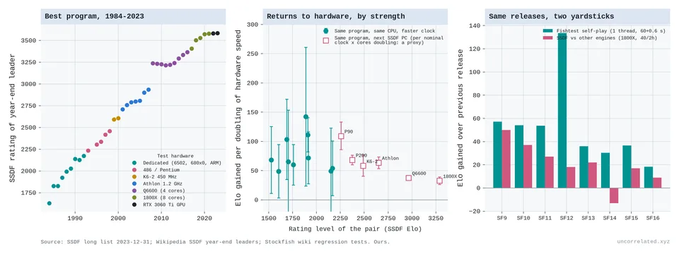
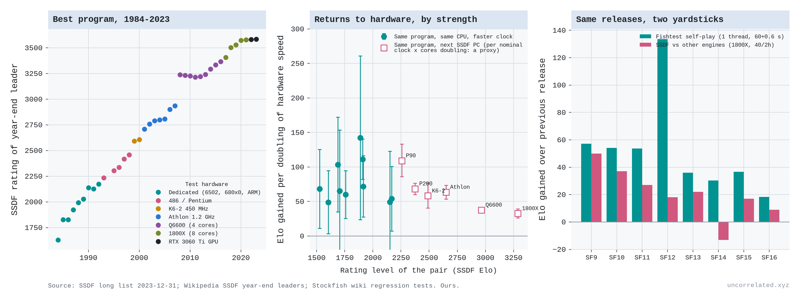
Figure 17: Left: the strongest program each year on the Swedish Chess Computer Association's rating list, by test hardware. Middle: Elo gained per doubling of hardware speed, from the same program tested on two machines, against playing strength. Right: Stockfish releases scored two ways: self-play on fixed hardware, and the SSDF list against other engines. Sources: SSDF; Stockfish regression tests.

• Chess shows what happens when the measuring stick saturates. Running the same program on a machine twice as fast was worth about 65–75 Elo points at ratings below about 2,200 (a median of 67 over ten pairs of tests, though individual pairs ranged from 49 to 142). Across hardware generations up to about 2,600 it was worth 58–109 points per doubling. That is log-linear, since Elo is itself a logarithmic scale. "Twice as fast" here means clock speed times cores, a rough proxy.
  • Near the top, at 3,000–3,300 Elo, a doubling was worth about half that, roughly 35 points.
  • Part of this may be the yardstick: if strong engines draw more of their games, rating gaps compress. We did not measure draw rates, but the same Stockfish releases (versions 8 to 16) gained 420 Elo in self-play testing but only 167 against other engines on the rating list.
  • The lesson carries over to AI capability indices. Near a ceiling, a constant real improvement shows up as shrinking gains.

Four more cases from the frontier of physical science. Here the output is reach, measured as digits of precision or as orders of magnitude of energy, sensitivity or plasma performance, so the gains per doubling can be compared with the computing cases above.

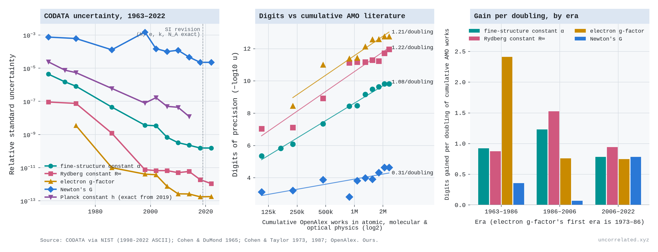
The fundamental constants

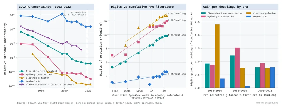
Figure 18: Left: relative standard uncertainty of five fundamental constants in each CODATA adjustment, 1963–2022 (log scale); the dashed line marks the 2019 SI revision, which made h exact. Middle: digits of precision against the cumulative literature of atomic, molecular and optical physics in OpenAlex, with logarithmic fits. Right: digits gained per doubling of that literature, by era. Sources: CODATA via NIST; Cohen & DuMond 1965; Cohen & Taylor 1973, 1987; OpenAlex.

• Measuring the constants of nature tracks the logarithm closely. Every few years the CODATA task group publishes recommended values of the fundamental constants, with their uncertainties (Cohen & DuMond, 1965; Cohen & Taylor, 1973; Cohen & Taylor, 1987; Mohr & Taylor, 2000; Tiesinga et al., 2021; Standards & Technology, 2024). The fine-structure constant α, which sets the strength of electromagnetism, went from a relative uncertainty of 4.4 × 10⁻⁶ in 1963 to 1.5 × 10⁻¹⁰ in 2022: about 29,000 times more precise.
  • Over the same years the cumulative literature of atomic, molecular and optical physics, the field that does this work, grew from about 106,000 to 2.3 million works in OpenAlex, 4.5 doublings. That is 1.08 extra digits of α per doubling (95% CI 1.03–1.13). The Rydberg constant and the electron's magnetic moment give about 1.2. The logarithmic and power forms fit about equally well, and the linear form loses badly (ΔAIC 28). Against this input the curve, if anything, bends slightly upward (p = 0.04); against the whole physics literature it is straight.
  • Between the endpoints of each era, α gained 0.92, 1.23 and 0.78 digits per doubling over 1963–86, 1986–2006 and 2006–22. In calendar time the last era was half as fast as the others, 0.41 digits a decade against about 0.9. The field's output of papers also stopped growing in OpenAlex after 2006, so the gain per doubling fell much less than the gain per decade. That is what the logarithmic law predicts, though the flat recent literature may partly reflect how OpenAlex classifies papers.
  • Newton's gravitational constant G is the exception in the same tables. Over the same 59 years it became only about 34 times more precise, 0.31 digits per doubling, and in 1998 it went backwards. The recommended value kept its 1986 value "but its uncertainty is about a factor of 12 larger", because one laboratory's careful result was "in severe disagreement with most other values" (Mohr & Taylor, 2000, p. 426). In 2018 the 16 measurements still disagreed enough that their uncertainties had to be enlarged by a factor of 3.9 (Tiesinga et al., 2021, p. 025010-6). Gravity is weak, there are few experiments, and each brings its own systematic errors, so effort does not accumulate the way it does for α.

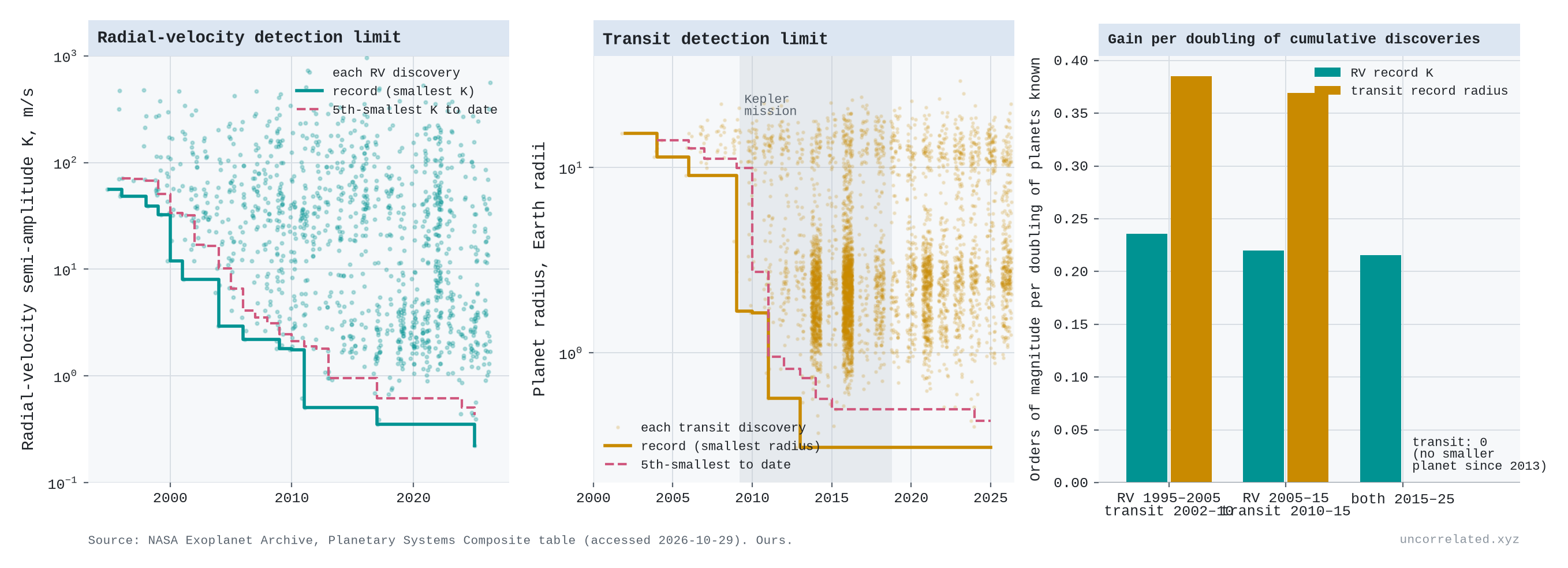
Planet hunting

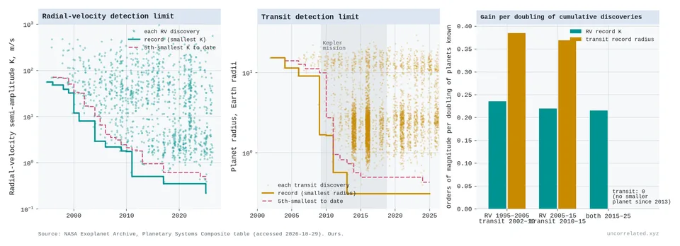
Figure 19: Left: the radial-velocity semi-amplitude K of each planet discovered by that method, with the smallest to date and the fifth-smallest to date. Middle: the same for planet radius among transit discoveries, with the Kepler mission shaded. Right: orders of magnitude gained per doubling of the cumulative number of planets known. Source: NASA Exoplanet Archive, Planetary Systems Composite table, accessed 2026-10-29.

• Planet hunting by radial velocity follows an experience curve. The method detects the wobble a planet induces in its star. In NASA's archive the smallest wobble behind a discovery fell from 56 m/s for 51 Pegasi b in 1995 to 0.22 m/s for Barnard e in 2025 (Institute, 2020).
  • Against the cumulative number of planets found, the gain between endpoints is strikingly constant: 0.24, 0.22 and 0.22 orders of magnitude per doubling over 1995–2005, 2005–15 and 2015–25. The logarithmic form beats the power form by ΔAIC 57 and the linear form by 69. Fitted within each decade, the gains are 0.26, 0.25 and 0.15, so the last decade may be slowing. Against the exoplanet literature, the 2015–24 gain falls to 0.13 from about 0.33.
  • Planets found are an output as well as an input, so this is an experience curve like Wright's law, not a causal estimate. The record also depends on target choice: the latest record holder orbits Barnard's Star, one of the Sun's nearest neighbours.
  • The transit method shows the other pattern. It watches for a star dimming as a planet crosses it. The smallest planet found this way shrank from 15 Earth radii in 2002 to 0.31 (Kepler-37 b) in 2013, and has not moved since. The seven smallest transiting planets in the archive were all found by the Kepler space telescope, which has since been retired. Since 2013 there have been more than 4,400 transit discoveries, including about 1,000 by its successor TESS, and none was smaller. More effort with the same class of instrument bought more planets but no further reach.

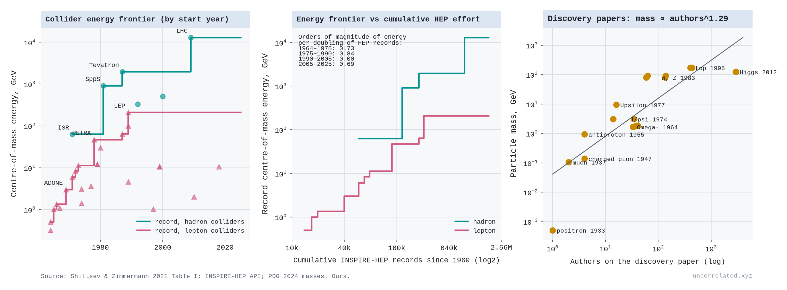
Particle colliders

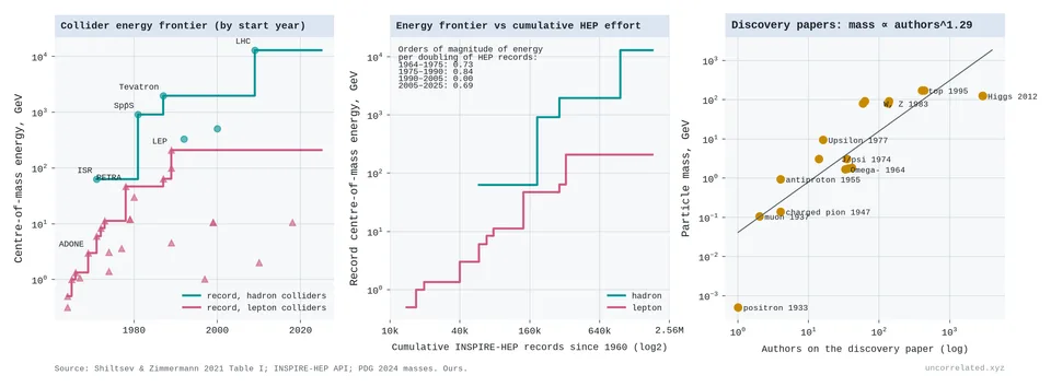
Figure 20: Left: maximum centre-of-mass energy of each collider against its start year, with the records for hadron and lepton colliders. Middle: the records against the cumulative number of particle-physics records in INSPIRE since 1960; inset, orders of magnitude gained per doubling, by window. Right: mass of particles against the number of authors on their discovery papers, with a log-log fit. Sources: Shiltsev & Zimmermann 2021, Table I; INSPIRE-HEP; Particle Data Group 2024.

• Particle colliders show a sawtooth whose teeth grow further apart. The record collision energy rose from 0.5 GeV in 1964 to 2 TeV at the Tevatron (1987) and 13 TeV at the Large Hadron Collider. Shiltsev and Zimmermann note that until the early 1990s it "increased on average by a factor of ten every decade" (Shiltsev & Zimmermann, 2021; arXiv:2003.09084v1, p. 3).
  • Against the cumulative particle-physics literature (INSPIRE-HEP, 2026), each doubling bought about 0.77 orders of magnitude of energy over 1964–90 and 0.34 over 1990–2025 (pooling the windows in the figure's inset). The 1990–2005 window bought nothing, and the LHC is the only step since. No electron-positron collider has beaten LEP's 209 GeV. Over the whole period the curve bends down significantly, worse than logarithmic.
  • I date each machine by its start year, using its maximum energy from Shiltsev and Zimmermann's table. Several machines, LEP and the LHC among them, reached their top energies years after they opened. Dating each step by when the energy was actually reached would move some steps later, but it would not remove the stall.
  • The input comes in lumps. A new energy record needs a single large machine that takes many years to build. Between machines the frontier stands still, however many physicists work on it.

Magnetic fusion

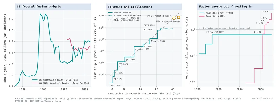
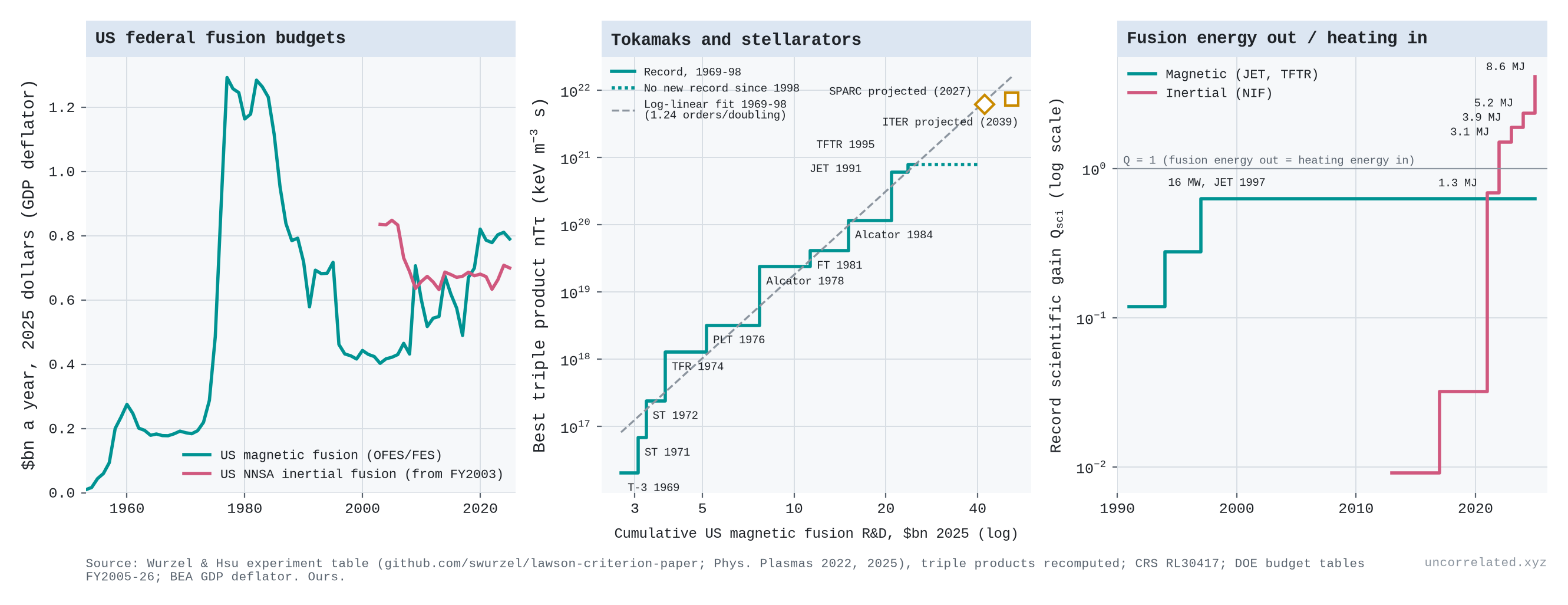
Figure 21: Left: US federal fusion budgets in 2025 dollars: magnetic fusion and, from FY2003, the NNSA's inertial fusion programme. Middle: the best triple product reached by tokamaks and stellarators against cumulative US magnetic fusion R&D, with the record holders, the 1969–98 logarithmic fit extended, and the SPARC and ITER design values placed at the cumulative spending projected for their target years at the 2021–25 rate. Right: record scientific gain (fusion energy out over heating energy in), magnetic against inertial, with NIF yields. Sources: Wurzel and Hsu's experiment table, triple products recomputed; CRS RL30417; DOE budget tables FY2005–26; BEA GDP deflator.

• Magnetic fusion was a steep log-linear case, and then stalled for thirty years. Its figure of merit is the triple product of a plasma's density, temperature and energy confinement time. On Wurzel and Hsu's consistent definition (Wurzel & Hsu, 2022; Wurzel, 2026), the record rose from 2.0 × 10¹⁶ keV m⁻³ s for the Soviet T-3 tokamak in 1969 to 7.9 × 10²⁰ for TFTR in 1995 (Wurzel & Hsu, 2022, p. 062103-21). That is about 40,000-fold in 26 years.
  • Against cumulative US magnetic fusion R&D over 1969–98 (Rowberg, 2000; U.S. Department of Energy, 2025), the gain is 1.24 orders of magnitude per doubling (95% CI 1.06–1.43). Against the world fusion literature in OpenAlex it is 1.33. On both inputs the logarithmic form fits best, with a mild downward bend. Lagging spending by ten years, since machines take about that long to build, gives 0.95.
  • Underneath, it is a sawtooth. By window, a doubling bought 1.61, 0.73 and 1.80 orders of magnitude over 1969–80, 1980–90 and 1990–98, with each jump arriving as a new generation of machines came online.
  • Then nothing. No tokamak or stellarator has beaten TFTR's 1995 record; the best since 1999 is JET's 2.2 × 10²⁰ in 2021. Since 1997, cumulative US spending has risen 66% and the world fusion literature 2.6-fold.
  • Gain shows the same stall. JET's 1997 record of 16.1 MW of fusion power, with a transient fusion amplification factor of 0.95 (Keilhacker et al., 1999, p. 209), gave a ratio of fusion power to input power of up to 0.64 (Keilhacker et al., 1999, p. 214), against TFTR's best of 0.27. No magnetic device has beaten it. JET did set new records for fusion energy per pulse, 59 MJ in 2021 and 69 MJ in its final experiments, both over about five seconds (News, 2024).
  • The stall is not a spending stall. Real US magnetic fusion spending peaked at $1.29 billion in 1977, then fell 5.2% a year to 1997, the twenty years in which half of the ten records were set. After 1997 it recovered at about 2.7% a year, and no record followed. As with colliders and transits, the frontier waits for the next, larger machine, and the US cancelled each candidate for it. The Mirror Fusion Test Facility was mothballed on the day it was dedicated in 1986 (Laboratory, n.d.). The Compact Ignition Tokamak was cancelled in the early 1990s (Rowberg, 2000, p. 11), the Burning Plasma Experiment by 1992 (Miley, 1992), and the Tokamak Physics Experiment after a 35% budget cut in 1996, which also ended TFTR in April 1997 (Rowberg, 2000, p. 11; Organization, n.d.). No deuterium-tritium tokamak larger than JET or TFTR has operated since. ITER now plans to start deuterium-tritium operation in 2039 (Organization, 2024, p. 2).
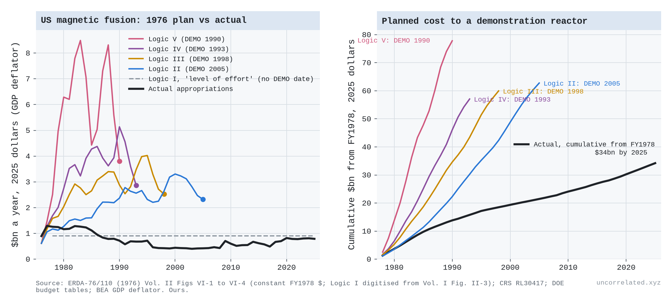
  • The planners priced progress in cumulative dollars. In 1976 the Energy Research and Development Administration set out five funding paths, its "Logics" (Research & Development Administration, 1976). The lowest, a flat "level of effort", was the one it warned might never produce a practical power plant. The other four reached a demonstration reactor in 1990, 1993, 1998 or 2005, depending on how fast the money came. Yet the three slower paths each needed about the same total, $57–63 billion in 2025 dollars from 1978. Actual US spending from 1978 to 2025 was $34 billion, 55% of what the slowest path needed by 2005. It fell below the "level of effort" line in 1987 and has stayed there. Of the machines the reference plan called for after TFTR (an ignition test reactor, an engineering test reactor, an experimental power reactor and the demonstration plant), none was built (Figure 22).
  • Extended forward, the 1969–98 dollar line passes close to the SPARC tokamak's design value (about 6 × 10²¹, listed for 2027 in Wurzel and Hsu's table). By 2039 the line reaches about twice ITER's design value of 7.4 × 10²¹. On this reading, fusion's progress has been paid for but not yet delivered. The reading depends on the input, though. Extrapolated against the world literature, the same line overshoots ITER more than tenfold, and the whole argument holds only if the machines perform as designed. Private money is a new surge of input. Fusion companies report $9.7 billion raised to 2025 and $4.5 billion more in the year to July 2026, more than five times the federal fusion programme's annual budget (Association, 2025; News, 2026). Even so, it adds less than half a doubling to the cumulative stock, so on this reading it should show up as new machines, SPARC first, before it shows up as records.

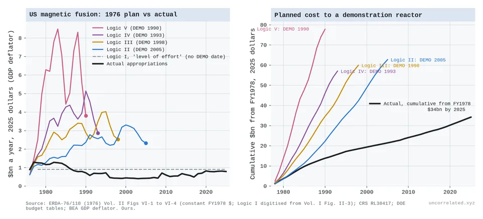
Figure 22: Left: annual US magnetic fusion budgets planned in ERDA's 1976 programme plan for Logics II–V, each line ending at its demonstration-reactor date, the flat Logic I "level of effort" path, and actual appropriations, all in 2025 dollars. Right: cumulative spending from FY1978 under each plan to its demonstration reactor, and actual. Sources: ERDA-76/110 Vol. II Figs VI-1 to VI-4 (Logic I digitised from Vol. I Fig. II-3); CRS RL30417; DOE budget tables; BEA GDP deflator. Our calculations.

Inertial fusion

• Inertial fusion crossed a threshold and did better than logarithmic. At the National Ignition Facility, lasers compress a capsule of fuel. On 5 December 2022 it produced 3.15 MJ of fusion energy from 2.05 MJ of laser energy delivered to the target. On 7 April 2025 it produced 8.6 MJ (± 0.45) from 2.08 MJ, a target gain of 4.13 (Laboratory, 2026).
  • Since 2013 the yield record has risen about 500-fold, while laser energy rose only from 1.5 to 2.2 MJ.
  • Real NNSA inertial fusion spending was flat: $0.84 billion in 2003, $0.70 billion in 2025. Against its cumulative total since FY2003, the yield record rose about three orders of magnitude per doubling, with a strong upward bend. That is over a single doubling, and without the pre-2003 budgets, so it is crude.
  • Ignition is a threshold with positive feedback. Once the fusion reactions heat the fuel themselves, yield climbs steeply. Before ignition, inertial fusion's triple product rose in steps, one for each new laser. Since 2017 it has been flat by that measure, because burning capsules reach higher pressure for a shorter time. Wurzel and Hsu note that the first ignition shot, on 8 August 2021, "tied the previous record" (Wurzel & Hsu, 2022, p. 062103-4).
  • Ignition also cost more than planned. NIF was expected to be finished in 2002 for about $2.1 billion (Office, 2000, p. 6); it began operating in 2009 at about $3.5 billion (Laboratory, n.d.).

Four direct tests

The cases above measure progress through a proxy: productivity, precision, approvals. Four older literatures measure it more directly, or measure a search whose pool is known to be finite. I re-ran each from public data.

Ideas: the breadth of a field against its literature

Staša Milojević measured the "cognitive extent" of a field as the number of distinct phrases in the titles of a fixed quota of its papers: 10,000 title phrases, about 3,000 papers (Milojevic2015, p. 5). Her conclusion: "While publication rates continue to grow exponentially, the cognitive domains expand on linear scales" (Milojevic2015, p. 14); "unlike the hundred- to a thousand-fold rise in the publication volume, the growth of cognitive extent is within a factor of few" [p. 11]. Linear growth in time while the literature grows exponentially is the same thing as linear growth in the logarithm of the literature, so her result is the thesis of this post in another form. The two come apart only when the growth of the literature changes speed.

I rebuilt her measure:

• Corpora. About 5,000–6,000 titles per five-year bin, sampled at random.
  • Physics: all American Physical Society journals.
  • Astronomy: ApJ, ApJS, MNRAS and AJ.
  • Biomedicine: English-language titles from OpenAlex, standing in for her PubMed.
• Phrases. Phrases were parsed by her rules: titles are split at punctuation and at general words, and each phrase is truncated to its last three words. Her list of general words is not published, so I used a standard stop-word list plus generic research words.
• Cleaning. Formula markup was stripped first. Left in, it creates thousands of repeated pseudo-phrases.

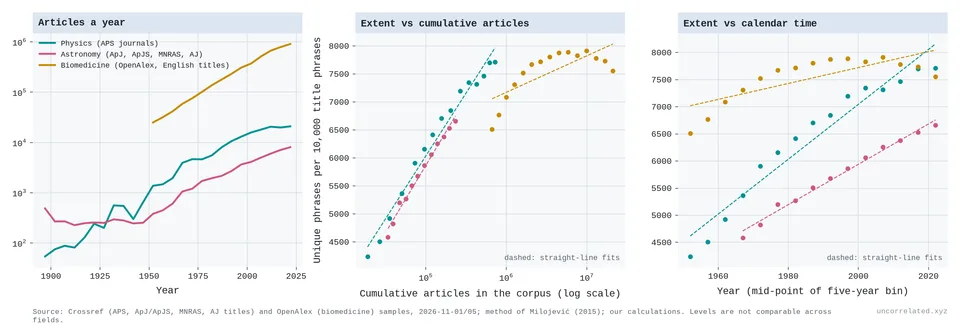
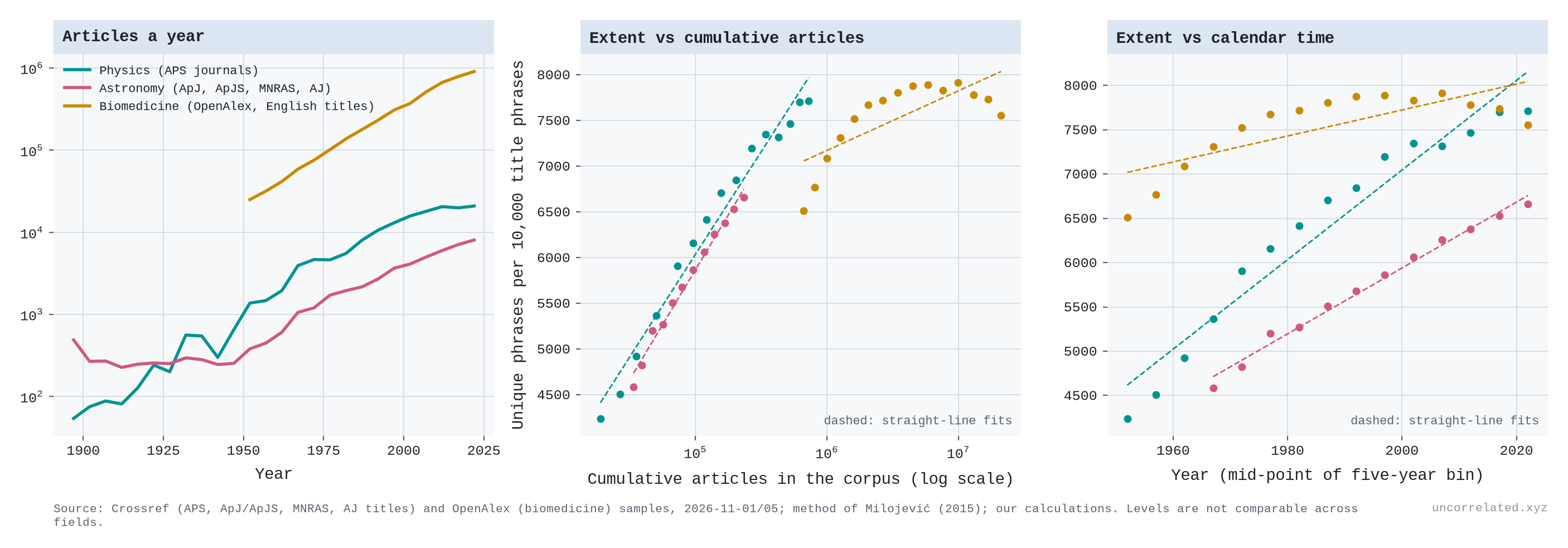
Figure 23: Left: articles a year in each corpus (log scale). Middle: unique phrases per 10,000 title phrases against the cumulative number of articles (log scale), with straight-line fits. Right: the same against calendar time. Levels cannot be compared across fields. Sources: Crossref and OpenAlex title samples; method of Milojević (2015); our analysis.

• Physics, 1950–2024. The literature grew 38-fold (5.3 doublings) and extent 1.8-fold, from 4,241 to 7,714 phrases. A straight line in the logarithm of cumulative articles fits better than a straight line in time (R² 0.98 against 0.94). At the largest quota the gain per doubling has been constant since 1990 (see below). The gain per doubling was 855 phrases in 1950–70, 637 in 1970–90, 441 in 1990–2005 and 517 in 2005–20. After 2005, APS output grew only about 1% a year: the gain per decade fell, but the gain per doubling did not.
• Astronomy, 1965–2024. The gain per doubling was about 940 phrases in 1965–80, 770 in 1980–95, 730 in 1995–2005 and 540 in 2005–20. Its literature grew at a steady rate, so time and the log of cumulative articles fit equally well.
• Biomedicine, 1950–2024. The breadth of biomedicine grew strongly until about 1980 and has not grown since 1990, although its literature has more than quadrupled. Per doubling, the gain was 867 phrases in 1950–65, 377 in 1965–80 and 150 in 1980–95; since then it has been about zero, and slightly negative after 2005. This is not just the spread of stock phrases such as "retrospective cohort study": counting those as general words leaves the plateau in place. An independent measure, the number of distinct OpenAlex research topics among 1,000 random papers, also stopped rising after 2005.

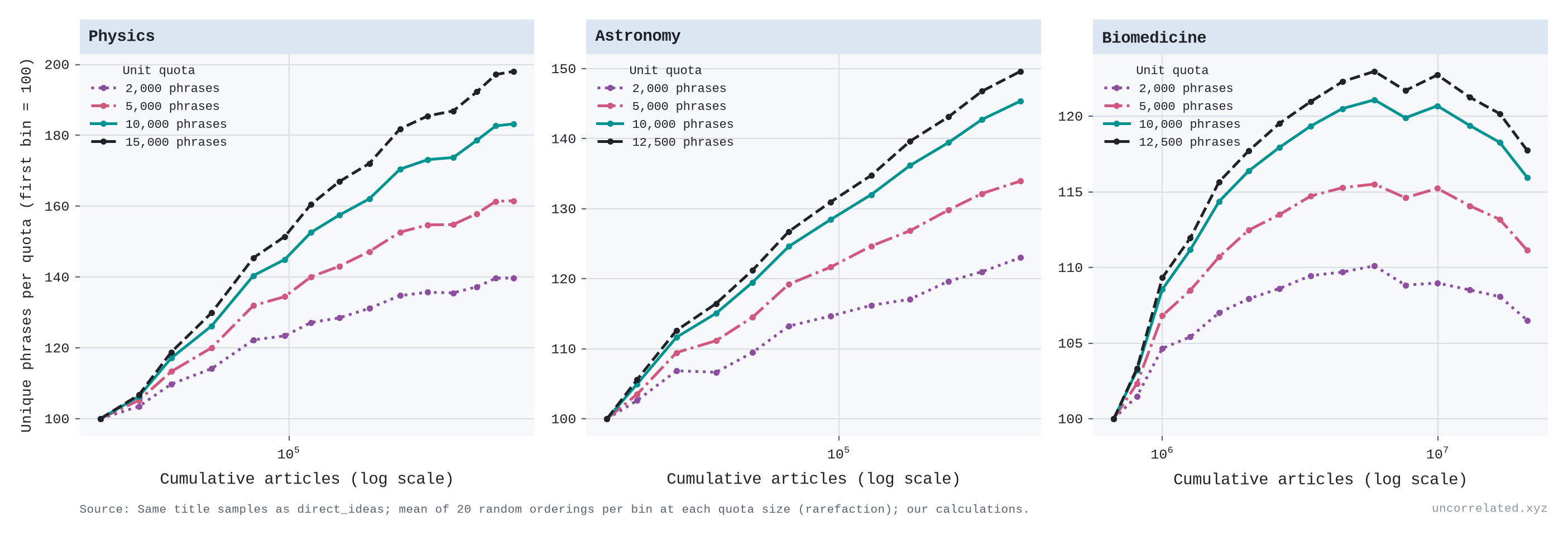
Is the bending real, or is the ruler running out? A quota of 10,000 phrases cannot hold more than 10,000 distinct ones, and physics and biomedicine now reach 77% and 79% of that. Milojević showed that this kind of saturation affects small quotas and is absent above 10,000 phrases (Milojevic2015, p. 8). Her own conversion between quota sizes reproduces our numbers to within about 2%. To check directly, I recounted every period at quotas from 2,000 phrases up to the largest every period's sample allows (12,500–17,500), averaging over 20 random orderings of the titles.

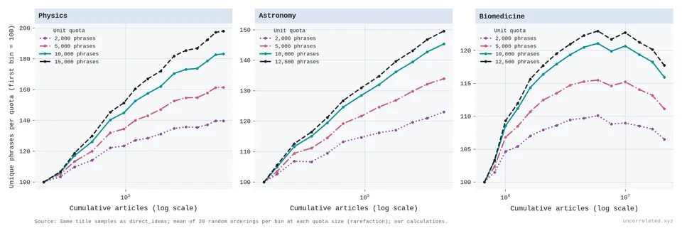
Figure 24: Unique phrases per quota, indexed to the first period, against cumulative articles, for quotas of 2,000 to 17,500 title phrases. Mean of 20 random orderings per period. Same samples as Figure 37. Our analysis.

• Physics. Part of its bend is the ruler. With the largest quota, the gain per doubling fell less, from about 1,300 phrases in 1950–70 to about 800 since 1990, rather than to 40% of its starting level. Since 1990 it has been constant per doubling at every quota: about 930 phrases in 1990–2005 and 940 in 2005–20 at 17,500. What remains is a faster expansion in the 1950s and 1960s, the post-Sputnik growth that Milojević also found.
• Biomedicine. The plateau is not the ruler. At every quota the breadth of biomedicine peaks in 1995–99, and by 2020–24 it is 3–4% lower, while its literature more than quadrupled. A ruler that is running out can flatten a rising line, but it cannot make it fall. The plateau may instead reflect what our sample counts as biomedicine (OpenAlex's topic labels) or a shift towards clinical studies with formulaic titles. It is a real feature of these titles, not of the method.

Experts: the Nobel survey

Patrick Collison and Michael Nielsen asked 93 physicists to judge 1,370 pairs of Nobel-winning discoveries, and ran similar surveys in chemistry and medicine. A decade's score is the probability that its discoveries win a pairing (Collison & Nielsen, 2018). In physics, every decade from the 1940s to the 1980s scored below every decade from the 1910s to the 1930s. Fitted to the 1910s–1980s, physics loses 0.028 points per decade (95% CI 0.006–0.050). Chemistry (+0.004) and medicine (+0.024) show no trend. Over the same seven decades the physics literature doubled about six times. The survey ranks only each decade's best few discoveries, and on a relative scale, so it cannot show growth. What it shows is that the best discoveries per decade did not get bigger as the input multiplied, which is what a constant step per doubling with steadily growing input predicts. Work from the 1970s and 1980s is still being awarded, which may bias the recent decades.

Species: a pool we have not yet drained

Taxonomists are the classic fishery: catch per unit effort falls as the pool empties. Joppa, Roberts and Pimm found that species descriptions and the number of describers have both grown "essentially exponential[ly]" since about 1950, and that only the species described per taxonomist declines (Joppa et al., 2011, p. 551). Their model, with an efficiency trend and a finite pool, predicted that the number of flowering plants should grow by "between 10 and 20 per cent" (Joppa et al., 2011, p. 554).

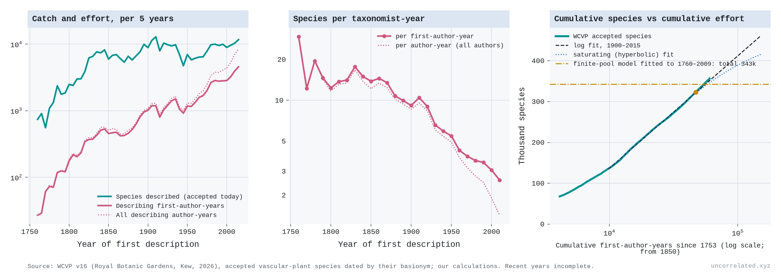
I used Kew's World Checklist of Vascular Plants (version 16, 2026), which covers 358,420 accepted species, each dated by its first description (Govaerts et al., 2021). Effort is the number of distinct describing authors each year, summed.

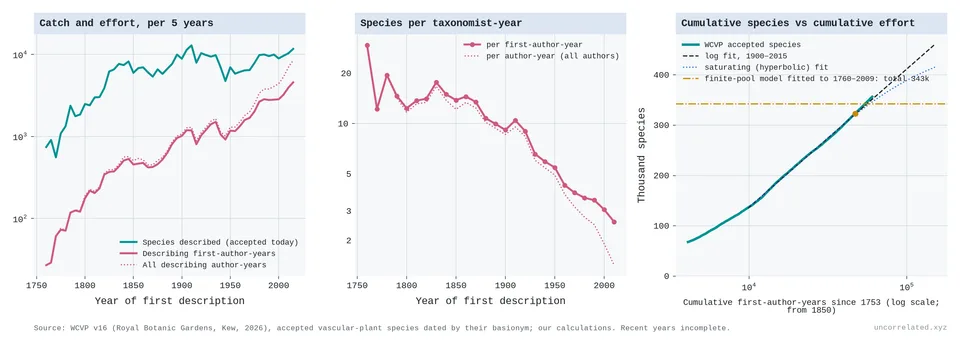
Figure 25: Left: species described (accepted today) and describing author-years, per five years. Middle: species per taxonomist-year by decade. Right: cumulative species against cumulative first-author-years (log scale). The dashed line is the logarithmic fit for 1900–2015, the dotted line a saturating fit, and the dash-dot line the total implied by Joppa et al.'s finite-pool model fitted to data up to 2009 (the dot marks 2009). Source: WCVP v16, Royal Botanic Gardens, Kew. Our analysis.

• The catch per unit of effort fell about five-fold, from 13.8 species per first-author-year in the 1850s to 2.6 in the 2010s, while authors per description rose from 1.1 to 1.8.
• Per doubling of cumulative effort, the catch has not fallen. The gain was 83,000 species in 1900–50, 76,000 in 1950–80, 86,000 in 1980–2000 and 92,000 in 2000–15. Counting the authors of every name, including those later sunk as synonyms, gives 80,000–93,000. Fitted to 1900–1976 with first-author effort, the logarithmic form forecasts 1977–2015 better than a saturating one (0.8% against 3.4% error). Counting all co-authors, whose numbers per description have risen, a saturating form does slightly better (2.6% against 2.9%).
• The finite-pool forecast has been overtaken. Fitted to data up to 2009, Joppa's model implies that 6% of vascular plants remained to be described. In 2010–24 botanists described 10% more (33,217 species). For monocots the model predicted 10.5% and 15.8% were described; for orchids, 4.8% and 18.4%. WCVP now lists more monocots and orchids than Joppa et al.'s own predicted totals (82,256 against 80,901; 30,990 against 28,894). Refitted to 2019, the model again says the pool is nearly empty.

The falling catch per botanist is not evidence that the pool is running out. A constant gain per doubling of cumulative effort implies it: if each doubling buys the same number of species, the yield per unit of effort must fall. The pool of plant species is surely finite, but the data are still on the straight part of the curve. There are two caveats. Recent names have had less time to be found to be synonyms, so the recent counts will shrink somewhat (Costello et al., 2013, p. 413). And effort is counted by its own successes.

Oil: a pool running dry

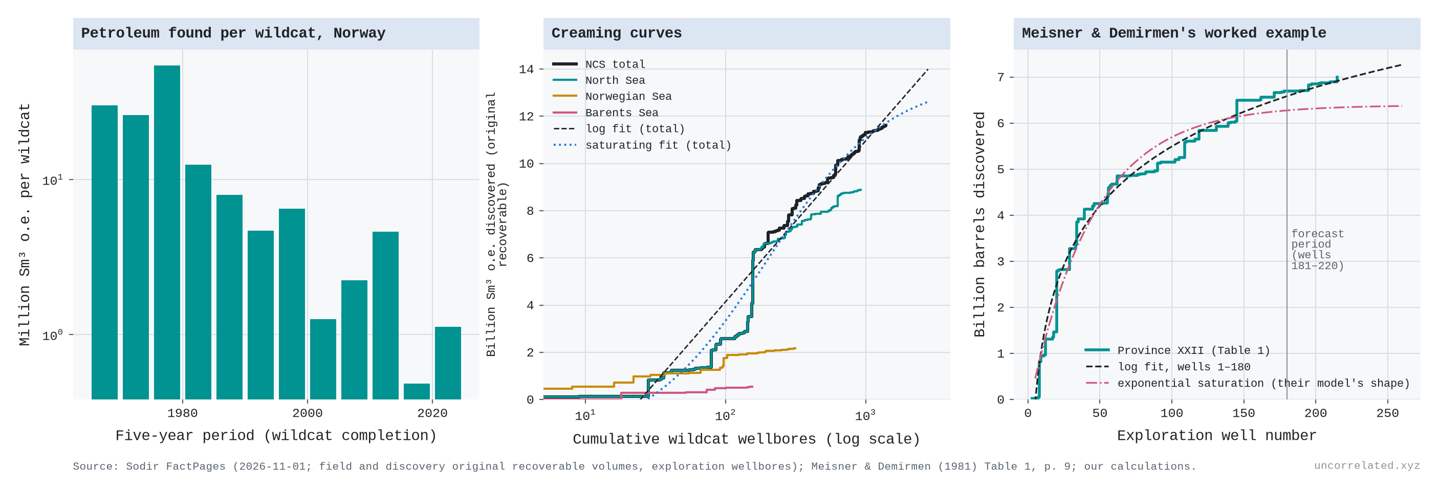
Petroleum geologists call it creaming: the big fields are found first, because "with each discovery the chance of making another discovery is reduced" and the industry is "generally capable of finding the larger fields early in exploration" (Meisner & Demirmen, 1981, p. 3). Meisner and Demirmen's worked example, a province of 220 exploration wells, is a good test of forecasting. Fitted to the first 180 wells, a logarithmic curve forecasts 373 million barrels from the last 40, a saturating (hyperbolic) curve 220, and their Bayesian model 281. The actual figure was 305.5 (Meisner & Demirmen, 1981, Table 1 p. 9, p. 17; our analysis).

For a full basin, I used the Norwegian Offshore Directorate's FactPages: 1,413 exploration wildcats since 1966, and the original recoverable volumes of 139 fields and 91 undeveloped discoveries, 11,617 million standard cubic metres of oil equivalent in all (about 73 billion barrels).

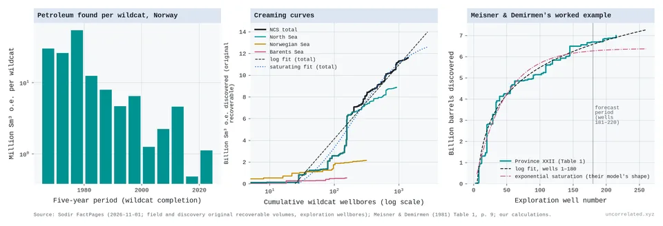
Figure 26: Left: oil and gas found per wildcat well, by five-year period (log scale). Middle: cumulative original recoverable volume against cumulative wildcat wells (log scale), for the whole shelf and each sea, with logarithmic (dashed) and saturating (dotted) fits to the shelf total. Right: Meisner and Demirmen's province XXII with fits to wells 1–180. Sources: Sodir FactPages, 1 November 2026; Meisner & Demirmen (1981), Table 1. Our analysis.

• More than half the volume was found by the first 200 wells. The first 200 of 1,413 wildcats found 57% of everything found to date; the first 700 found 88%. Volume per wildcat fell from 39 million m³ in 1966–79 to 1.1 in 2020–25.
• The step per doubling shrinks. On the whole shelf a doubling of cumulative wildcats bought 3,375 million m³ in 1975–85, about 2,000 in 1995–2015 and 777 in 2015–25. In the North Sea it bought 3,096, then 1,443, 454, 1,695 (Johan Sverdrup, found in 2010) and 452.
• Saturating curves forecast better. Fitted to the first two-thirds of discoveries, a hyperbolic curve forecasts the rest with 1.1% error, a logarithmic curve with 2.6%. The hyperbolic fit implies about 2,000 million m³ left to find.

This is what a finite pool looks like: worse than a constant step per doubling, within each sea. The shelf as a whole bends less because new seas were opened. Drilling in the Norwegian and Barents Seas began in 1980, and the Barents Sea, the youngest, is still on its logarithmic stretch. The creaming curve also flatters the early wells. Each field's volume is dated to its first well, so later satellite finds (193 discoveries in 63 fields) and later upward revisions (+18% for the fields already booked in 2004) are credited to the early wells.

What the cases say

So "a constant gain per doubling" is the middle case, not a universal law. Some outputs do better than log for long stretches, as crop yields did against public R&D. Some do worse, as single-thread chips have since about 2004. (US life expectancy looks worse after 2010, but its rich-country peers kept their gains per doubling.) New drugs were log-linear for forty years and have done better since 2010. Precision measurement and radial-velocity planet hunting, both done by many mid-sized laboratories, come closest to a constant gain per doubling. Where one large instrument holds the frontier, as with colliders, transiting planets and magnetic fusion, progress stops between instruments however much else is spent. Inertial fusion shows the opposite, a threshold that, once crossed, made progress better than logarithmic. What the cases share is that sustained progress needed input that kept growing, or a new paradigm when it didn't: single-thread chips gave way to parallel chips and GPUs.

Most of these series rise by a roughly constant step per doubling of their input, or a slightly shrinking one: the breadth of physics and astronomy, plant species, and the Nobel scores, which stayed flat per decade while input doubled every decade or so. Two fall clearly below the line. Oil, the one pool that is plainly being drained, does so basin by basin. The breadth of biomedicine has stalled since the mid-1990s. That is not the measure reaching its ceiling. It is either a real narrowing of what biomedicine writes about relative to how much it writes, or an artefact of how the corpus is defined. The distinction that matters is not the shape of the curve over the range seen so far. It is whether there is an independent ceiling (geology for oil, heritability for genetics) and how close to it we are. A large pool seen from far away (plants) looks the same as an open frontier (ideas in physics) until enough of it has been drained for each doubling to buy visibly less.

S4. Genomics

The cleanest real-world example of "subtler effects need exponentially bigger samples" is human genetics.

In the 2000s, candidate-gene studies reported sizeable effects of single genes on traits like depression, in samples that were small by later standards. Almost none survived. Border et al. tested the 18 most-studied depression candidate genes in very large samples and concluded that "as a set, depression candidate genes were no more associated with depression phenotypes than noncandidate genes" (Border et al., 2019, p. 376).

Then genome-wide association studies (GWAS) scaled up by orders of magnitude, and real associations started appearing in their thousands, each one tiny. I analysed every study in the NHGRI-EBI GWAS Catalog (1.2 million association rows).

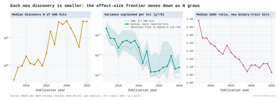
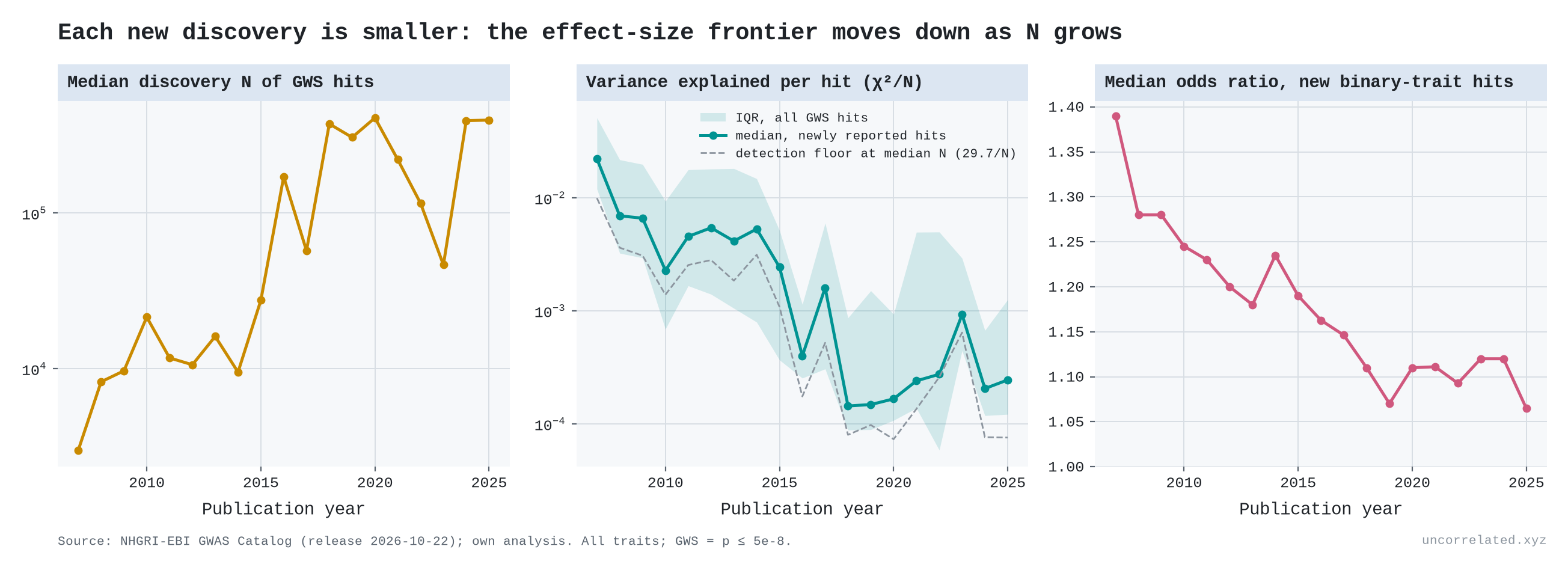
Figure 27: Median discovery sample size of genome-wide-significant hits (left); variance explained per newly reported hit, with the detection floor implied by sample size (middle); median odds ratio of new binary-trait hits (right). Each new discovery is smaller: the effect-size frontier moves down as N grows.

• Sample sizes: the median discovery sample behind a newly reported hit rose from about 3,000 people (2007) to about 390,000 (2024–25).
• Variance explained: the median per new hit fell about 100-fold, from 0.022 to roughly 0.0002. Much of that fall is mechanical, because bigger samples can detect smaller effects: at genome-wide significance, a study of N people can detect a variant only if it explains more than about 30/N of the variance. The informative part is that new hits keep appearing at every new detection floor, in steady or growing numbers: there was always a lot of real effect hiding at ever smaller sizes.
• Odds ratios: the median odds ratio of new disease hits fell from 1.39 (2007) to 1.12 (2024) and 1.07 (2025).

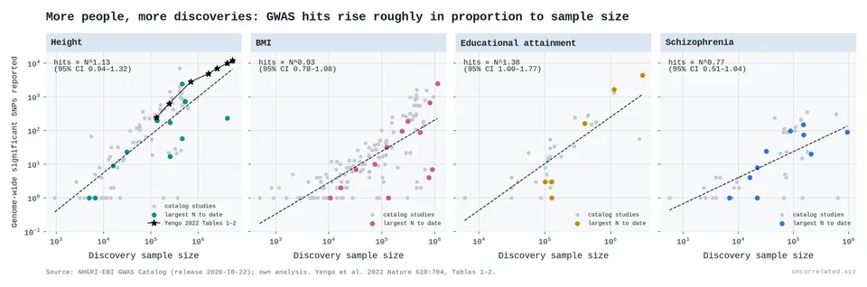
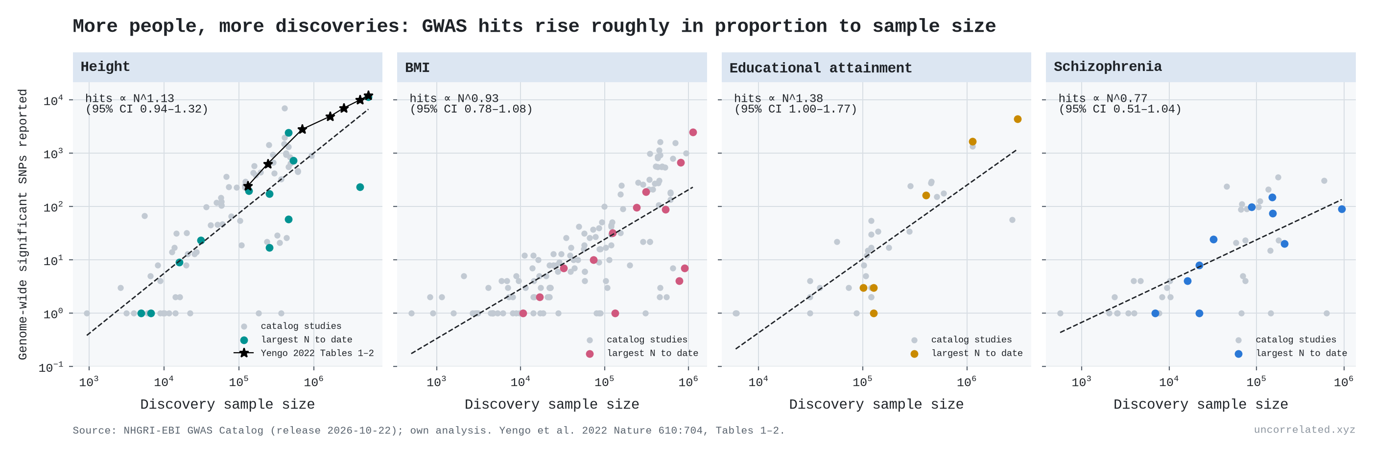
Figure 28: Genome-wide-significant hits against discovery sample size for height, BMI, educational attainment and schizophrenia. The height panel includes Yengo et al.'s 2022 analysis.

Height is the textbook case. In Yengo et al.'s consistent re-analysis (Yengo et al., 2022, Tables 1–2):

• 130,000 people yield 240 significant SNPs;
• 700,000 yield 2,794;
• 5.4 million yield 12,111, which account for "nearly all of the common SNP-based heritability".

The hit count grows roughly in proportion to sample size, so in hits alone returns are not logarithmic. But the value of each extra hit collapses. In Yengo's own words, going from 2.5 million to 4 million people added thousands of SNPs, "but the absolute increase in prediction accuracy is less than 2.7%" (Yengo et al., 2022, p. 710).

Hits are a count. What a hit is worth is better measured by how well the genome predicts the trait. Geneticists measure that with a polygenic score: add up every variant's estimated effect and check how much of the variation in a new sample the total explains.

Theory says this curve has a ceiling. Accuracy can never exceed the share of variation the measured variants carry, the "SNP heritability". A breeding-genetics formula from 2008 says how fast you approach it: accuracy depends on sample size times heritability, divided by the number of effective loci (Daetwyler et al., 2008, p. 2). Plotted against log sample size, that formula gives an S-curve.

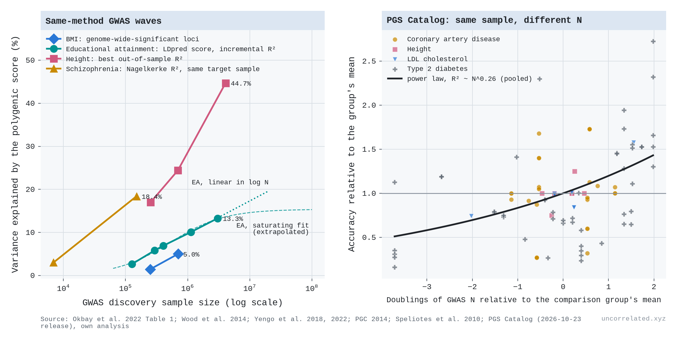
The educational attainment consortium re-scored every one of its GWAS waves with the same method and the same test samples (Okbay et al., 2022, Table 1):

• 127,000 people: the score explains 2.6% of the variation in years of schooling;
• 294,000: 5.8%;
• 405,000: 6.9%;
• 1.1 million: 10.1%;
• 3.0 million: 13.3%.

Each doubling of the sample added 2.6, then 2.4, 2.2 and 2.2 percentage points. That is a straight line in log N, and it fits better than the textbook S-curve (residual sum of squares 3.6 times smaller), which says the gain per doubling should already have fallen to about 1.3 points [our analysis]. The education score also picks up family environment: controlling for parents' scores "roughly halves" the association (Okbay et al., 2022, p. 438), so its ceiling is not a pure genetic one. Height has gone further, with improving methods along the way: 17% at 250,000 people, 24% at 700,000, and 45% at 4 million (Wood et al., 2014; Yengo et al., 2018; Yengo et al., 2022, p. 5). That 45% is about 90% of height's ceiling, which is why the last 1.5 million people bought so little.

In the PGS Catalog, there are 35 comparisons in which the same evaluation sample was scored with genetic studies of different sizes (13 publications; height, LDL cholesterol, coronary artery disease, type 2 diabetes). A power law with exponent 0.26 fits best, then a straight line in log N, with the textbook saturating curve last; it wins in only 12% of bootstrap draws. The gain per doubling shows no sign of shrinking (quadratic term +0.03, p = 0.19). Only coronary artery disease leans towards saturation [our analysis]. The Catalog is thin for this question, and method and sample size improve together, so the education series remains the clean test.

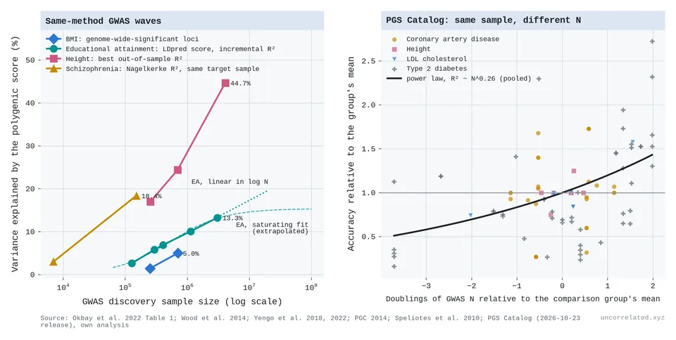
Figure 29: Left: variance explained by polygenic scores against GWAS sample size, for waves analysed with consistent methods (height mixes methods). Educational attainment gains about 2.3 points per doubling. The dashed curve is the saturating textbook fit; the dotted line extends the straight-line fit. Right: in the PGS Catalog, the same evaluation sample scored with GWASs of different sizes (35 comparisons, 13 publications). Accuracy keeps rising per doubling with no sign of tapering. Sources: Okbay et al. 2022; Wood et al. 2014; Yengo et al. 2018, 2022; PGC 2014; Speliotes et al. 2010; PGS Catalog (release 2026-10-23). Our analysis.

So prediction is a finite-pool case: a fixed amount of heritability, approached log-linearly. The S-curve's flat top is real for height and still ahead for most traits. The middle stretches over decades of sample size because effects come in every size, and each size class needs its own tenfold more people (Zhang et al., 2018).

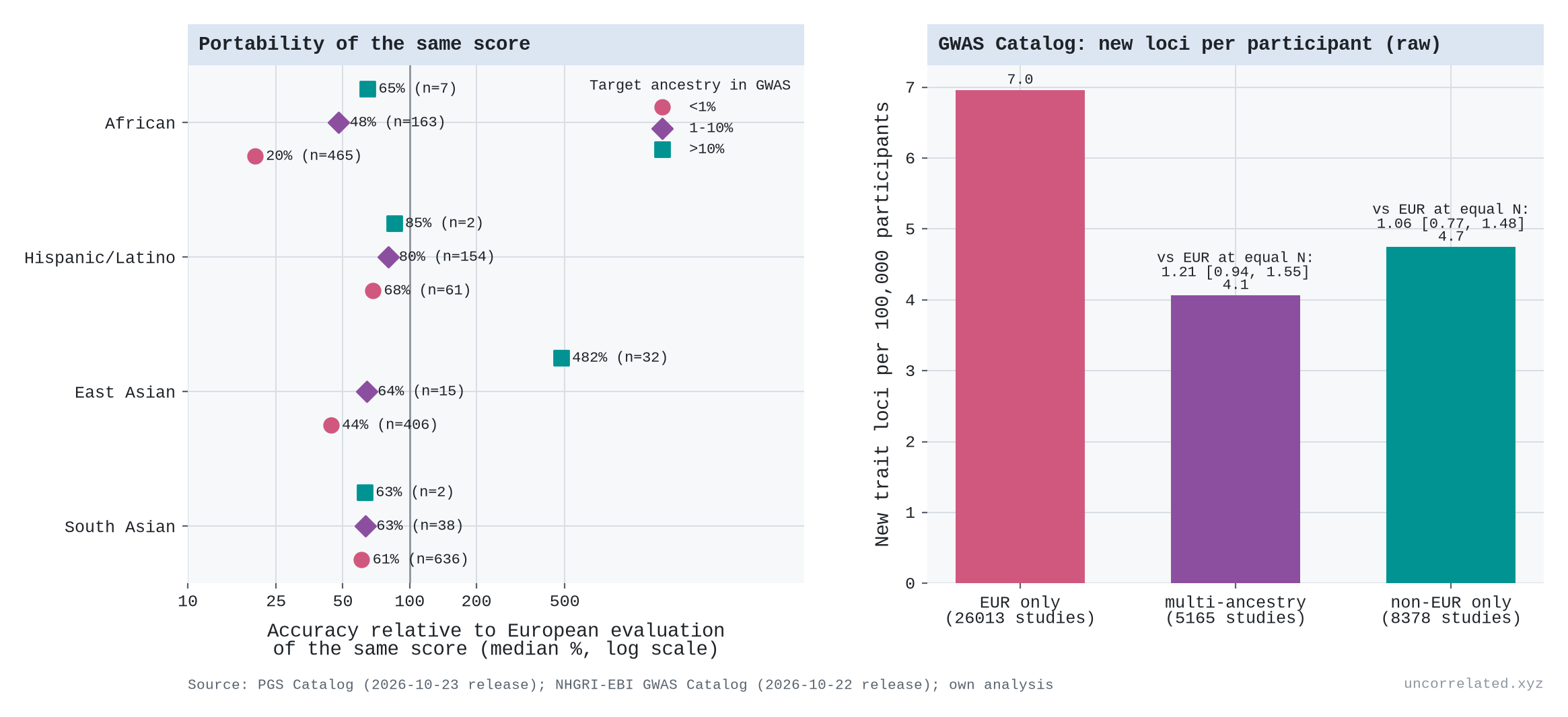
Which participants count? Here the "trials" are people, and the analogue of new robot environments is new ancestries. For finding loci, a new ancestry is not worth more. In the GWAS Catalog, at equal sample size and controlling for trait, year and what was already known, studies of non-European samples report about as many new loci per participant as European ones (rate ratio 1.06, 95% interval 0.77 to 1.48; multi-ancestry 1.21, 0.94 to 1.55). Within a trait, each doubling of the loci already known cuts the rate of new ones by about 24% [our analysis]. For prediction, new ancestries are worth far more, but only for the people they come from. Scores built from European samples lose most of their accuracy in other groups: in our pull of the PGS Catalog, a score's accuracy in African-ancestry samples is about 20% of its European accuracy when under 1% of the GWAS was African, and about 48% at 1 to 10% (comparing different scores, so suggestive) [our analysis]. Privé et al. find 18% in a Nigerian-ancestry group across 245 traits (Privé et al., 2022, p. 5). Yengo's height study puts a price on it. 1.5 million more Europeans added under 2.7 points of accuracy; about 1 million non-Europeans added over 3.4 points of multi-ancestry accuracy (Yengo et al., 2022, p. 7).

That is the robot result again: more of the same saturates, and coverage of where you want to predict pays. It has limits, though. Mixing ancestries at a fixed sample size did not help in one large test (Privé et al., 2022, p. 7), diverse meta-analyses still mostly help Europeans because they are still mostly European, and for educational attainment, most of the accuracy gap in African-ancestry samples is not explained by genetic differences between groups (Okbay et al., 2022, p. 440).

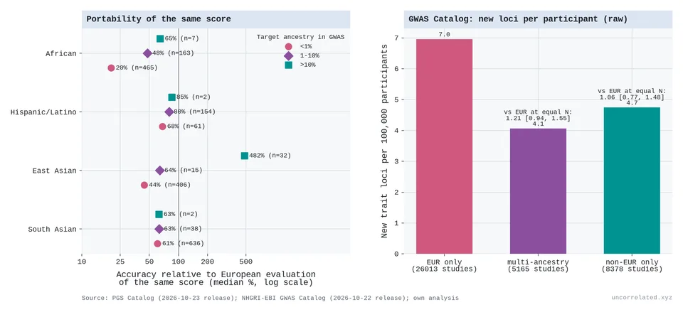
Figure 30: Left: accuracy of the same polygenic score in non-European samples relative to European samples, by how much of the development GWAS came from the target ancestry (PGS Catalog, median over score-evaluation pairs). Right: new trait loci per 100,000 participants by discovery-sample ancestry (GWAS Catalog, raw rates); labels give the rate ratio against European-only studies at equal sample size, trait and prior knowledge. Our analysis.

That is the counts-versus-value distinction from the main post again: discoveries stay cheap to count and get ever more expensive to make matter.

S5. Machine learning and robotics

Neural scaling laws are the most precisely measured case of all. Kaplan et al. found language model loss falling as a power law in parameters, data and compute, with exponents of about 0.076, 0.095 and 0.050 (Kaplan et al., 2020, eqs. 1.1–1.3). With a compute exponent of 0.05, each tenfold increase in compute cuts loss by only about 11%.

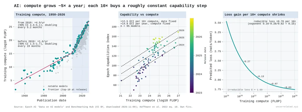
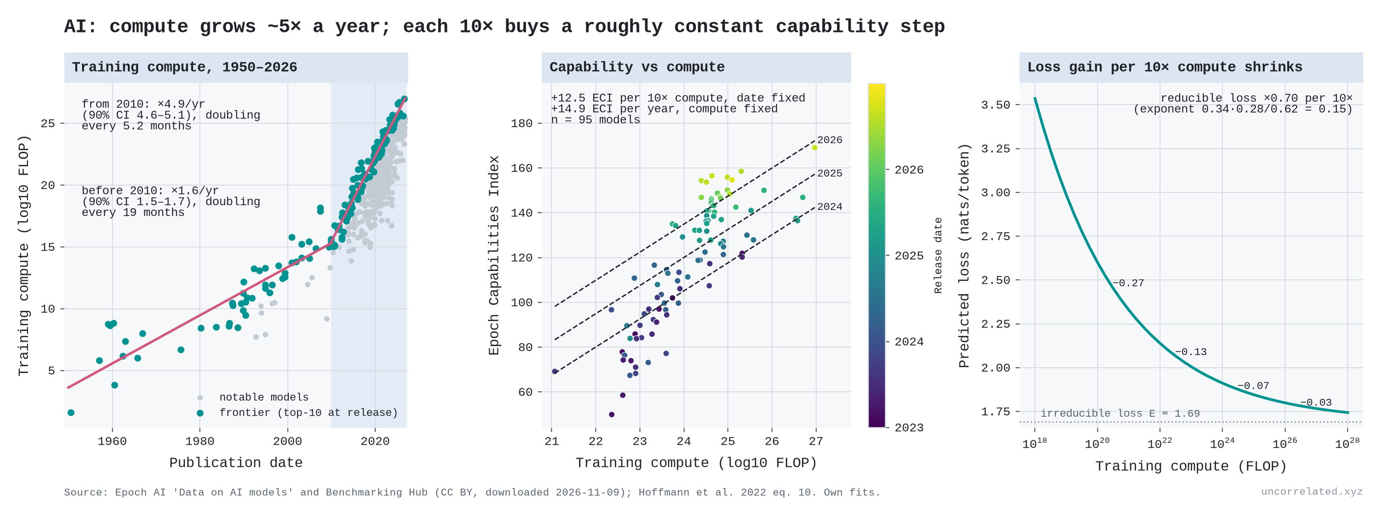
Figure 31: (a) Training compute of notable AI models since 1950, with the frontier trends before and after 2010. (b) Epoch Capabilities Index against compute, coloured by release date. (c) Chinchilla's fitted compute-optimal loss against compute.

From Epoch AI's open model data:

• Compute growth: frontier training compute grew 4.9× a year over 2010–2026 (90% CI 4.6–5.1×), doubling roughly every five months. Epoch's own published figure is 5.3× a year for 2010–2024 (90% CI 4.9–5.7×), which it summarises as 4–5× a year (Sevilla & Rold{\'a}n, 2024); over that same window we get 4.9×, the difference coming from a newer data vintage and our own selection of the top ten models. Before 2010, the same frontier grew about 1.6× a year (90% CI 1.5–1.7×), doubling every 19 months. Sevilla et al.'s earlier analysis gave doubling times of about 20 months before 2010 and about 6 months in the deep-learning era (Sevilla et al., 2022).
• Shrinking gains: on Chinchilla's fitted loss curve (Hoffmann et al., 2022, eq. 10), each 10× of compute multiplies the reducible loss by about 0.70. The absolute improvement per 10× keeps shrinking: 0.27, 0.13, 0.07, 0.03 nats, starting from 10²⁰, 10²², 10²⁴ and 10²⁶ FLOP.

Strictly, this is a power law, not a logarithm: the gain per tenfold of compute keeps shrinking. Over the range anyone has trained, though, it is the same story of steeply rising input for steady progress, and progress has stayed steady because compute has grown about fivefold every year.

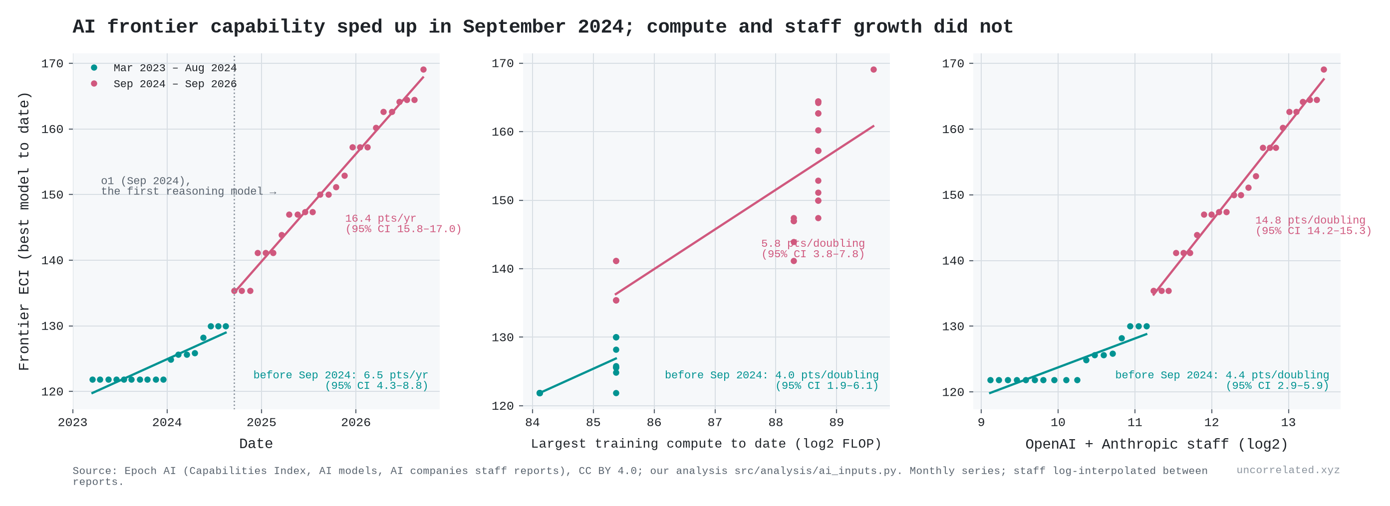
There is a complication: algorithms also improve. Ho et al. estimate that the compute needed to reach a given level of performance "halved approximately every 8 months" over 2012–2023 (Ho et al., 2024, p. 1). The transformer alone was worth "nearly two years of algorithmic progress" (Ho et al., 2024). These observational estimates may be biased: labs choose how much compute to use partly on the basis of algorithmic quality the data don't record (Whitfill, 2025). So effective input has grown even faster than physical compute. Epoch's capability index tells the same story from the other side. Holding compute fixed, it rises about 15 points a year (against about 12.5 points per tenfold of compute), and over 2023–26 the capability gained per physical FLOP has not been falling. That is the strongest evidence against the thesis anywhere in this post. My reading is that the progress was still bought with input, but much of that input was ingenuity rather than hardware, and ingenuity is hard to count. Some of it can be counted, though. Epoch's tally of reported headcounts (AI, 2026) shows the leading labs growing exponentially too:

• OpenAI: from 52 staff at the end of 2016 to about 4,500 in March 2026, roughly 60% a year.
• Anthropic: from about 50 in 2022 to 5,300 in September 2026, roughly tripling every year.
• DeepMind: from 75 in 2013 to 1,000 in 2021, about 40% a year, before its merger with Google Brain.

These are whole-company counts, not researchers alone. At Anthropic at the end of 2024, research and development accounted for 521 of 915 staff. So they are rough, but they make the point. The human input at the frontier labs has been multiplying by 1.4 to 3 times a year.

So is capability log-linear in these inputs? Over the last two years, not in staff; for compute the evidence is weak.

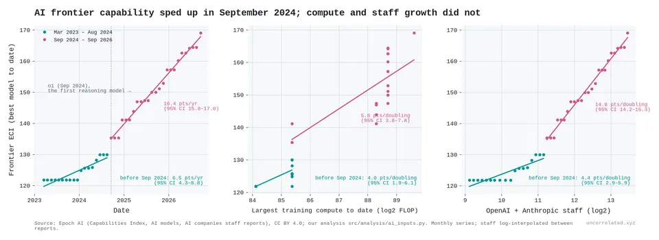
Figure 32: The best Epoch Capabilities Index score to date, monthly, March 2023 – September 2026, against time (left), the largest training run to date (middle) and OpenAI and Anthropic's combined staff (right). Lines are fitted separately before and after September 2024; slopes with 95% CIs. Our analysis of Epoch AI data.

From March 2023 to August 2024 the best score on Epoch's index rose about 6.5 points a year. From September 2024, when OpenAI released o1, the first of the "reasoning" models, it rose about 16 points a year. Two of the inputs we can count kept roughly their usual pace across that break. The largest training run grew a little faster after it (about 1.7 doublings a year, against 1.3 before), and the two labs' combined staff a little slower (1.1 against 1.5). So the gain per doubling of staff jumped, while the gain per doubling of compute barely moved:

• Per doubling of OpenAI and Anthropic's combined staff: from about 4 index points to about 15 (95% CIs 2.9–5.9 and 14.2–15.3).
• Per doubling of the largest training run: from about 4 to about 6, a difference within the margin of error (95% CIs 1.9–6.1 and 3.8–7.8).

The third input did speed up. In Epoch's estimates, the cost of the most expensive training run barely grew before the break (0.2 doublings a year) and then grew about 1.35 doublings a year, mostly in one step, from about $53 million in mid-2024 to $366 million in early 2025 (2023 dollars). Per doubling of that cost the gain fell: about 13 index points before and 6 after, though the earlier figure rests on a single step in cost and is imprecise (95% CI 8–17). Against money spent at the frontier, capability did not speed up across the break.

The "before" window is also short. It starts at GPT-4, and the index did not move in its first ten months, so the slow early rate depends partly on where the window starts.

So capability has grown faster than the logarithm of staff, and perhaps of compute, but not of the frontier training budget. I can see three readings:

1. The input moved off the books. Reasoning models get large reinforcement-learning runs after pre-training, and they spend far more compute while answering. Neither shows up as training compute. The labs' total compute bills, which include both, grew fast: OpenAI's from about $5.8 billion in 2024 to about $16 billion in 2025, and Anthropic's from about $2.5 billion to about $7 billion (AI, 2026). These are reported figures and partly projections. The jump in the cost of the largest training run points the same way.
2. A one-off new technique, like the transformer before it. A log-linear world allows occasional jumps. The question is whether 16 points a year persists or settles back.
3. The index itself. The ECI is a statistical scale stitched together from many benchmarks. A point at the top may not mean the same as a point at the bottom.

The window is only three and a half years. If the first reading is right, the thesis survives with a bigger input than the one we measure. If the pace holds without any input growing to match, AI is the first real break from the pattern in this post. It is the case I'll be watching most closely.

Robots are the next test, and they show the same shape so far. Their training sets have grown faster than text did: 10,000 hours of robot data for Physical Intelligence's π0 in 2024, half a million hours for Generalist's GEN-1 and over a million hours of human video for Dyna-2 in 2026 (Black & others, 2024; AI, 2026; Robotics, 2026). In controlled experiments, success on unseen homes and objects rose by a roughly constant 12–17 percentage points for each doubling of the number of distinct training environments, over five doublings (Lin et al., 2025; Intelligence, 2025). More demonstrations in the same environments stopped helping after about 800. At industrial scale, Dyna reports zero-shot accuracy on robot data rising only from 7% to 16% over a thousand-fold increase in hours of video, though that is a company figure, not a peer-reviewed one. The input that behaves logarithmically is diversity, not hours. And because a success rate is capped at 100%, each doubling can at best remove a fixed share of the failures that remain: 28–44% per doubling in these experiments.

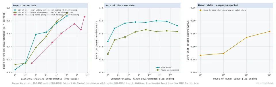
Figure 33: Left: score on unseen environments against the number of distinct training environments (Lin et al., two tasks; π0.5 with the number of training samples held fixed). Middle: score against demonstrations for a fixed set of environments. Right: Dyna-2's zero-shot action accuracy on robot data against hours of human video (company-reported). Sources: Lin et al. 2025, Tables 4–11; Physical Intelligence 2025, Fig. 8 (digitised); Dyna Robotics 2026, Fig. 2. Our fits.

Why would returns be logarithmic?

The intuition I started from goes like this. A model first learns the strongest, simplest regularities in its data. It then moves to subtler interactions between features, then to interactions between interactions. Each layer is rarer and needs more data to resolve. If each layer is worth roughly the same improvement, but each costs a multiple more data than the last, you get a constant gain per doubling of data.

Michaud et al. formalised a version of this as the "quantization model": skills come in discrete chunks learned in order of how often they are used, and "a power law in use frequencies explains observed power law scaling of loss" (Michaud et al., 2023, p. 1). Hutter (Hutter, 2021) and Bahri et al. (Bahri et al., 2024) give related accounts.

To make the intuition concrete, I built a toy simulation: a target function made of successive layers of k-th order interactions, learned by a model that adds layers as data allow.

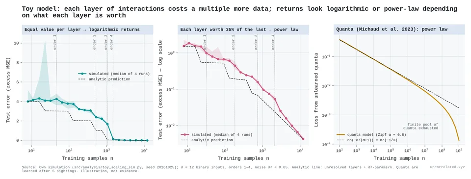
Figure 34: Toy simulation, an illustration and not evidence. (1) When every interaction layer is worth the same, test error falls in roughly equal steps per multiple of data: logarithmic returns. (2) When each layer is worth a fixed fraction of the one before, error falls along a straight log-log line: a power law. (3) A Michaud-style "quanta" model with Zipf-distributed skill frequencies gives a power law.

What the simulation shows is useful:

• The cost side is the same in every version. Each next layer of subtlety costs a roughly constant multiple of data.
• The value side decides the shape. Equal-value layers give logarithmic returns, a constant gain per doubling. Layers of shrinking value, or Zipf-distributed skills, give a power law.

So "exponentially more data for each next layer" holds literally only when layers are counted on a log scale. Stated that way, it is the same claim as the rest of this post.

It is also Arrow's point from S1, sixty years on. Repeating the same problem teaches less each time, and the same holds for data. Training a language model on the same text up to four times is almost as good as training on new text; beyond that the value of repeats decays, and after about sixteen passes it is mostly gone (Muennighoff et al., 2023, pp. 1, 4, 7). Robots show the same thing with environments rather than text (Figure 33). In both learning curves and scaling laws, what accumulates is informative examples, and new kinds of example count for more than more of the same.

S6. Teams, training, prizes and discovery lags

If each frontier step needs exponentially more input, no single person can supply it. The prediction is that the lone genius fades and science becomes a team sport.

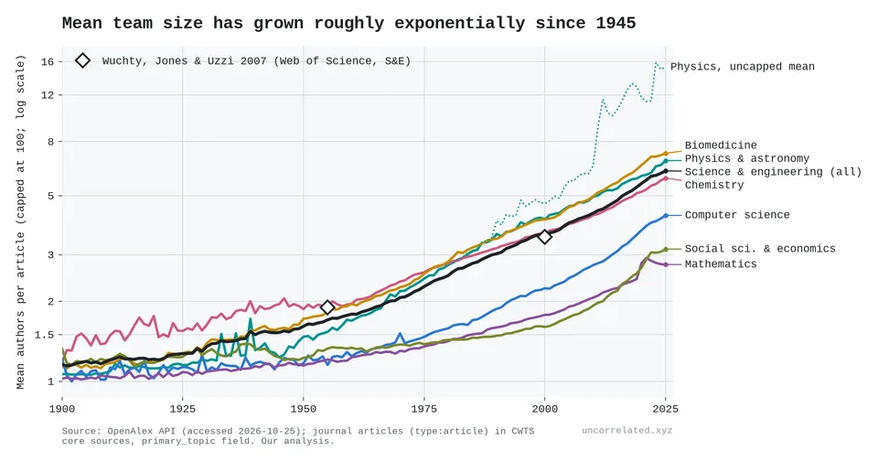
Figure 35: Mean authors per article by field, 1900–2025 (capped at 100 to stop thousand-author physics papers dominating). Diamonds: Wuchty, Jones and Uzzi's two benchmark points.

From exact counts of every journal article in OpenAlex's core sources:

• Team size: mean authors in science and engineering rose from 1.70 (1955) to 3.62 (2000) to 6.60 (2025); capping papers at 100 authors, as in the figure, gives 6.21. That is a steady 1.8% a year since 1945, a straight line on a log scale. Wuchty, Jones and Uzzi, using Web of Science, reported growth "from 1.9 to 3.5 authors per paper over 45 years" (Wuchty et al., 2007, p. 1). Our figures for mathematics match theirs closely: 1.21 → 1.78 authors against their 1.22 → 1.84.
• Solo authorship: the share of solo papers in science and engineering fell from 57% (1955) to 22% (2000) to 5.8% (2025). Even in mathematics, 79% of papers now have co-authors.

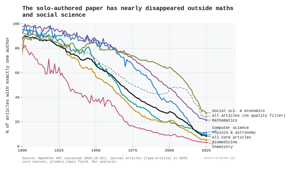
Figure 36: Share of articles with exactly one author, by field, 1900–2025.

Particle physics is the extreme case. By INSPIRE's author counts, the 1933 paper reporting the positron had one author; the two 1974 papers announcing the J/ψ had 14 and 35; the top quark papers of 1995 had 436 and 403; and the Higgs boson papers of 2012 had 2,932 and 2,900 (INSPIRE-HEP, 2026). Across 18 discovery papers for 13 particles, the particle's mass rises roughly as the number of authors to the power 1.29 (95% CI 0.74–1.84; right panel of Figure 20). Restricted to the accelerator era (1964 on, 14 papers), the exponent is 0.83 (0.45–1.20). Heavier particles needed bigger teams, but the Higgs, lighter than the top quark, needed about seven times as many people. The papers are our own selection, so treat the exponent as an illustration, not a law.

Nobel prizes show the same thing:

Award period	Prizes	Share awarded to one person	Mean laureates	Mean age at award
1901–1950	127	76%	1.29	51
1951–2000	150	32%	2.03	57
2001–2026	78	9%	2.55	68

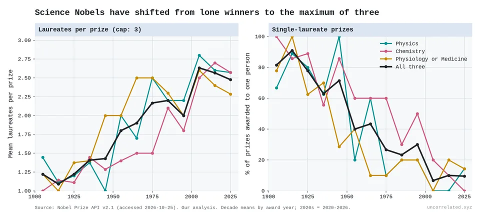
Figure 37: Mean laureates per science Nobel prize (left) and share of prizes awarded to a single person (right), by decade.

Using Jones and Weinberg's data on when the prize-winning work was done (Jones & Weinberg, 2011), which cover prizes up to 2008:

• Age at the work, averaged by prize decade, rose from 39 to 42. That understates the shift, because the most recent work hasn't been rewarded yet. Counted by when the work was done, physics laureates' mean age at their prize-winning achievement since 1980 is 48 (Jones & Weinberg, 2011) (47 in our copy of their data). Indexing their data by the decade in which the work was done, and pooling all three science prizes, mean age at the work was 36–40 in every decade from the 1900s to the 1970s, then 44 for work done in the 1980s and 47 for the 1990s. The share of prize-winning work done before 40 fell from about half to two-thirds in the decades before 1950 to 38% for the 1980s and 22% for the 1990s. The recent decades rest on fewer cases (48 and 18), and they are censored, because much recent work has not been rewarded yet. In physics, great achievement by age 40 fell to 19% of cases by 2000, under a third of its 1900 rate; in chemistry it fell towards zero.
• The wait from discovery to prize grew from 13 to 23 years, and in physics from 10 to 26.

So laureates are doing their great work later in life and waiting longer for the prize. The first is what the burden of knowledge predicts: it takes longer to reach the frontier. The second is what you'd expect if eminent work keeps arriving while the prize count stays fixed.

How much longer is the climb?

If knowledge piles up, everyone has more to learn before they can add to it. Jones calls this the "burden of knowledge" (Jones, 2009). On the thesis, the frontier deepens with the log of the literature, so the climb should lengthen by a constant amount per doubling, not in proportion. The science literature in OpenAlex doubled about eight times between 1900 and 2025.

• Age at entry rises by about a year per doubling. US inventors' age at first patent rose 0.66 years a decade in 1985–99 (Jones, 2009, p. 291). Mathematicians' age at their first top-journal article went from 28 to 33 between 1950 and 2013 (Brendel & Schweitzer, 2019, p. 143). Nobel laureates' age at their highest degree rose about 4 years a century (Jones, 2009, p. 284; reproduced in our analysis). Converted to the same unit, these give 0.7–1.5 years per doubling of the literature.
• Not in proportion. A burden proportional to the stock would have multiplied training time about 250-fold. Instead, the median US time from bachelor's degree to PhD in the physical sciences was 6 years in 1936 and 6.7 in 2024 (Tuckman et al., 1989, p. 507; Science & Statistics, 2025, Table 1-12).
• Papers read wider, not deeper. The median article cites 39 works, up from 6 in 1950: roughly the square root of the literature's growth. The average cited work is still about 10 years old, as it was in 1930 [our analysis of OpenAlex].
• More knowledge, bigger teams. When Soviet mathematics reached the West after 1990, team sizes rose 8% more in the subfields where Soviet work was strongest (Agrawal et al., 2016, p. 101).

But:

• Demography explains a lot. About 40% of the eight-year rise in age at great achievement reflects an ageing population (Jones, 2010, p. 6).
• The recent jump is partly censored. Work from the 1980s and 1990s counts only if it was rewarded by 2008. Through 1980 the rise is about 3 years a century.
• Institutions can reverse it. US time to PhD fell in every science field after 1994, and inventors have got younger since the late 1990s (Jung & Ejermo, 2014; Kaltenberg et al., 2023). The rising age at a first NIH research grant (38 to 45 for physicians, 1980–2013) mostly reflects a queue for jobs (Daniels, 2015, p. 313).
• Not unique to this thesis. Jones's own growth model, where narrower specialisation and bigger teams absorb the burden, predicts the same slow rise (Jones, 2009). What fits the thesis specifically is the shape: a constant cost per doubling, not a cost in proportion to what is known.

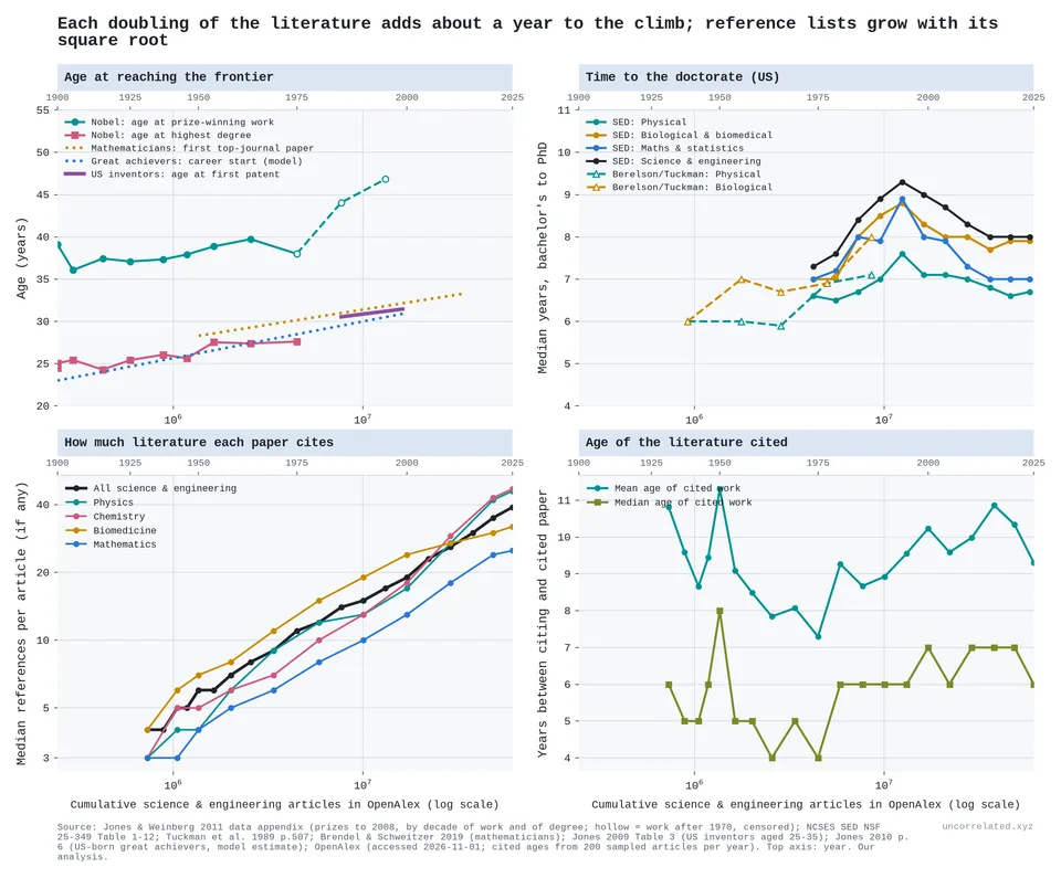
Figure 38: Time to the frontier against the cumulative science and engineering literature in OpenAlex (log scale; top axis: year). Top left: Nobel laureates' mean age at prize-winning work and at highest degree, by decade (hollow = censored), with published trends for mathematicians, great achievers and US inventors. Top right: median years from bachelor's degree to PhD in the US, by field. Bottom: median references per article, and the age of cited works (200 sampled articles a year). Sources: Jones and Weinberg 2011; NCSES; Tuckman et al. 1989; Brendel and Schweitzer 2019; Jones 2009, 2010; OpenAlex; our analysis.

Do discoveries come sooner once they are possible?

If effort keeps growing, more people and more attention sit on every problem. So the wait between a discovery becoming possible and being made should shrink, and grow less erratic. Most lags agree on the first half, but not all:

• Tool to discovery. Across Krauss's 761 major discoveries, the average gap after the enabling tool was 30 years in the 1800s, 21 and 10 years in the two halves of the 1900s, and 6 years in 2000–2022 (Krauss, 2026, p. 7). The recent figure flatters: a discovery made after 2000 is counted only if it was recognised by 2022, and tools are often dated to the "improved" version built for the discovery itself.
• Invention to adoption. Across 15 technologies, each decade of later invention cut the average cross-country adoption lag by about 5 years, from 120 years for steamships to 8 for the internet (Comin & Hobijn, 2010, Table 2; our fit).
• Product to imitation. For 46 US product innovations, the wait between a new product's launch and the rush of competitors fell from about 23 years for products launched before 1930 to about 5 for those launched after 1940 (Gort & Klepper, 1982, p. 640); a later study of 46 innovations puts it at almost 33 years around 1900 and 3.4 years in 1967–86 (Agarwal & Gort, 2001). Holding the observation window fixed, the fall is smaller but still there: 13 to 6 years (our analysis of Gort & Klepper, 1982, Table 2).
• Independent rediscovery. In Ogburn and Thomas's 1922 list of multiple discoveries, the median gap between the first and second independent discoverer fell from 7 years before 1700 to zero in 1850–99, and gaps of a decade or more fell from 39% to 7% (Ogburn & Thomas, 1922; our transcription).
• But not invention to first use. A 1966 study for the US automation commission found the time from technical feasibility to commercial development falling from 30 years (1885–1919) to 9 (1945–64) (Lynn, 1966, p. II-40). That rests on 20 innovations, grouped by when development began, which favours short recent lags; grouped by when each innovation became feasible, its fall disappears, though on very few cases. Larger lists, consistently dated, show no trend. Within the same observation window, Enos's 35 inventions, from Newcomen's engine to Dacron, averaged 6 to 9 years from invention to first use in every era from the 1700s to the 1930s, and the Jewkes cases invented before and after 1910 both averaged about 13 years (Enos, 1962; Clark et al., 1981; our analysis). Some 19th-century inventions took far longer, such as the fluorescent lamp's 79 years, but later inventions had not had time to show such delays when these lists were compiled. The best-known claim of acceleration, Mensch's, depends on his early invention dates (Clark et al., 1981).
• But slowly, and the noise shrinks only in proportion. These lags halve roughly every 50–70 years, while US research effort has doubled about every 16. The spread of adoption lags stays almost exactly proportional to their mean, and in the product-launch lists the relative spread even grows (for competitors' entry, the ratio of standard deviation to mean rose from 0.5 to 0.8), so lags became shorter, not more predictable [our analysis]. Recognition went the other way: as above, the wait for the Nobel itself grew, and its spread widened (Jones & Weinberg, 2011; our analysis).
• Falling lags fit the thesis without singling it out. The lags that fell are mostly about spreading what already exists: adoption, imitation, rediscovery. Their own authors credit easier transfer of knowledge and bigger markets (Agarwal & Gort, 2001). Faster communication and purpose-built instruments explain more, and any model with growing effort predicts the fall. The step that more effort should speed most directly, getting a workable invention into use, did not get faster in the classic lists. The slowness is the telling part. Each doubling of effort cuts the lag by only 15–20%, where a doubling of eyes on every problem would halve it. That is another face of diminishing returns.

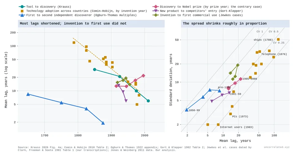
Figure 39: Left: mean lag in years (log scale) for Krauss's gap from enabling tool to discovery, by period of discovery (teal); Comin and Hobijn's cross-country adoption lags for 15 technologies, by invention year, with a log-linear fit (amber); the gap between the first and second independent discoverer in Ogburn and Thomas's list of multiples, with gaps capped at 23 years so every period has the same observation window (blue); and, the contrary case, the delay from prize-winning work to Nobel prize, by prize period (rose); the time from a new product's launch to the take-off in competitors' entry (Gort and Klepper's 46 US products, introduced by 1953, lags over 20 years dropped; purple); and the time from invention to first commercial use for the Jewkes et al. cases as dated by Clark, Freeman and Soete, by date of first use (olive). Right: standard deviation against mean for the same lags; dotted lines mark constant ratios of SD to mean. The spread shrinks roughly in proportion to the mean, not faster, and for the product and invention lags its relative size grows. Sources: Krauss 2026; Comin and Hobijn 2010; Ogburn and Thomas 1922; Gort and Klepper 1982; Clark, Freeman and Soete 1981 (our transcriptions); Jones and Weinberg 2011. Our analysis.

S7. The replication crisis and the death of genius

These two subsections back the main post's discussion.

The replication crisis

I think it is, and the mechanism is sample size. Run a thousand studies with a hundred people each, publish the ones that cross a significance threshold, and you get a literature full of large effects, many of them noise. Scale the samples up and the noise washes out. What is left is the real effects, and they are small. The replication projects show exactly this. Replicated effects come in at two-thirds of the original size or, more often, much less:

Project	Replications significant	Replication effect as share of original
Open Science Collaboration 2015 (psychology)	36% (vs 97% of originals)	about 0.5 (our recomputation from their data: 0.50)
Camerer et al. 2016 (economics)	61%	0.66
Many Labs 2	54%	0.25 (median d 0.60 → 0.15)
Cancer biology, 2021	43% of positive results	0.15 ("85% smaller")

Sources: (Collaboration, 2015; Camerer et al., 2016; Klein et al., 2018; Errington et al., 2021).

Ioannidis predicted this in 2005 (Ioannidis, 2005): small samples, flexible analysis and publication filters inflate the effects that get reported. Some famous findings were probably never real at all; others were real but much smaller than first claimed. Either way, the lesson for this post is the same. The effects still left to find are small, and finding them reliably takes samples orders of magnitude larger than the field used to run.

Genetics is the cleanest demonstration. Its candidate-gene era looked like early psychology: big effects from small samples that mostly didn't hold up. Its true effects were always tiny; the field only found them once samples grew by orders of magnitude. The best way to put it: low-hanging-fruit depletion in effect-size space. The effects that need small samples to detect are, by definition, the large ones, and the catalogue shows each new generation of hits sitting at the new detection floor. What remains requires millions of people per study.

The death of genius: eminence per unit of input

If the easy discoveries came first, fame per unit of input should fall. The most direct test uses the cross-verified database of 2.3 million notable people. I counted notable scientists, engineers and inventors by birth decade, then divided by different measures of input.

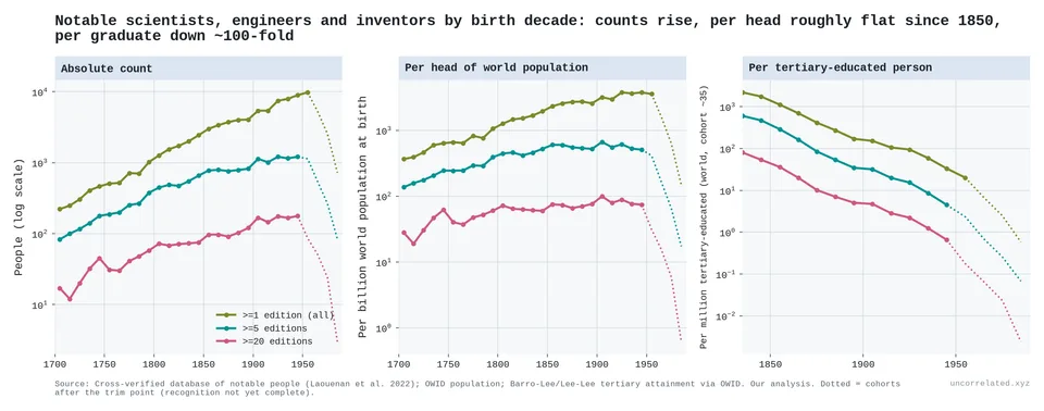
Figure 40: Notable scientists, engineers and inventors by birth decade. Absolute counts rise (left). Per head of world population, the count is roughly flat since about 1850 (middle). Per tertiary-educated person, it falls about 100-fold (right). Dotted segments are recent cohorts whose recognition is incomplete.

• Absolute counts rise across the whole period. This matches the earlier Huebner post on this blog, which found that notable innovators did not become rarer in absolute terms.
• Per head of world population, the count rises until about 1850 and then stays roughly flat. Restricted to people born in Europe and the Americas, it falls about 40% from its peak.
• Per tertiary-educated person, the closer proxy for scientific input, the count falls about 100-fold between cohorts born in the 1840s and the 1940s. Over that span the tertiary-educated population grew about 190-fold and the number of notable scientists 1.8-fold.

That last comparison fits "exponential input, roughly constant output", but it is suggestive rather than decisive. It is an upper bound on the decline, and it should not be read as a direct measure of research productivity.

Caveats:

• Fame is partly positional. If the number of famous-scientist "slots" grows more slowly than the number of scientists, eminence per scientist falls mechanically. This metric cannot separate "each scientist contributes less" from "fame is spread more thinly".
• Teams were always ahead at the top. Team papers have been about twice as likely as solo papers to reach the top 1% most-cited since the 1920s, and that ratio has risen only modestly. Solo authors' share of top papers collapsed mostly because solo papers became rare, not because solo work got worse.
• The early denominators are fragile. Tertiary attainment before 1900 is reconstructed from tiny shares (about 0.07% of the world in 1870), so the size of the 100-fold fall is uncertain, although its direction is not.
• Growing teams aren't proof on their own. Cheaper communication, authorship norms and capital-intensive science would all grow teams too.

The team and genius evidence is consistent with the thesis, not proof of it.

S8. China

If returns are logarithmic, a country pouring money into research should see diminishing returns. China did the opposite.

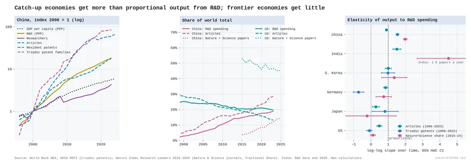
Figure 41: China's indices since 2000 (left); China and US shares of world R&D, articles and Nature+Science papers (middle); elasticity of research output to R&D spending, by country (right).

Since the late 1990s:

• Inputs: between 2000 and 2023, Chinese R&D (PPP) rose from $45 billion to $825 billion, about 13% a year, and researchers from 0.7 million to 3 million.
• Frontier output: China's elasticity of output to spending was 1.5 for triadic patent families (patents filed in the US, Europe and Japan; 1996–2022) and 2.0 for its fractional share of papers in Nature and Science (2015–24).
• Frontier vs volume: its Nature+Science share grew 17% a year over 2015–24, faster than its overall paper count (11% a year over 2015–23).

The frontier economies look completely different:

Country	Elasticity of Nature+Science share to R&D
US	0.11 (95% CI −0.04 to 0.26)
Japan	−0.23 (−1.91 to 1.45)
Germany	0.73 (0.28 to 1.18)
South Korea	1.35 (0.62 to 2.07)

The picture is messier than a clean frontier/catch-up split. The US is near zero. Japan's estimate is too noisy to say anything. Germany is clearly positive, though below proportional. Korea, which spends 4.9% of GDP on R&D, has an elasticity well above one on Nature+Science, but its share of the broader Nature Index has been flat and its articles per R&D dollar have stalled since 2015.

I think this sets the thesis's scope rather than refuting it. A catch-up country learns from the existing world stock of knowledge cheaply. Its returns are logarithmic in the world's frontier, not in its own spending, and the world frontier is far ahead of where its own effort started. Diminishing returns should bite hardest near the frontier, and the US, the clearest frontier economy, shows them most clearly.

Two caveats:

• The Nature+Science share is zero-sum. China's gains are partly other countries' losses, so a frontier country's near-zero elasticity partly reflects displacement.
• Chinese patent counts are inflated by filing subsidies: local subsidy programmes raised firms' patent counts by more than 30% (Dang & Motohashi, 2015). Triadic families correct for this only partly.

S9. Where the pattern breaks, and other objections

Where the pattern breaks

A constant step per doubling is the typical case. The exceptions matter as much as the rule.

• New tools bring bursts. Sequencing between 2007 and 2010 improved far faster than its learning curve, then returned to it. New drug approvals have run at about twice their old rate per doubling of R&D since 2010 [our analysis]. A new paradigm opens a fresh field of easy improvements.
• Thresholds. At the National Ignition Facility, inertial fusion crossed ignition in 2022. Its yield record has risen about 500-fold since 2013 on flat spending, because once the fusion reactions heat the fuel themselves, yield climbs steeply (Laboratory, 2026; our analysis).
• Giant machines. Where one large instrument holds the frontier, as with colliders and magnetic fusion, progress stops between machines however much else is spent.
• US productivity has barely declined since the 1980s. Research productivity in the aggregate US data has been roughly flat for four decades [our analysis; S2]. If that continues, the aggregate pattern describes 1930–1990 better than today.

AI since late 2024 is the other candidate exception. It is treated in S5.

Other objections

The mechanism is not identified. Several stories predict falling research productivity:

• Logarithmic returns: each increment costs more as the stock of knowledge grows. This is Rescher's view.
• Low-hanging fruit: the supply of easy ideas is finite, and the best ones were found first.
• The burden of knowledge: training takes longer, specialisation narrows and teams grow (Jones, 2009).
• Institutional drag: large fields fixate on canonical work (Chu & Evans, 2021), and big teams develop where small teams disrupt (Wu et al., 2019).

The aggregate data cannot tell these apart. Growing teams are consistent with the burden-of-knowledge channel, but they are not unique evidence for it. The rising age of prize-winning work, documented by Jones and Weinberg, points the same way.

The disruption decline is fragile. Park et al.'s widely reported finding that papers and patents are "becoming less disruptive" (Park et al., 2023) shrinks dramatically under scrutiny, at least for patents:

• Macher et al. find that correcting for truncation bias leaves only "a marginal decrease in the CD index over time", and that the number of highly disruptive patents has increased since 1980, "particularly since 2008" (Macher et al., 2024).
• Petersen et al. conclude that growing reference lists make the CD index "systematically biased and unsuitable for cross-temporal analysis" (Petersen et al., 2024).

I don't rely on it.

Huebner's innovation peak in 1873 rests mainly on a single history book's list (Huebner, 2005). The earlier replication on this blog, with a much larger database, found no absolute decline. The per-input view above is the version of his claim that survives: absolute output rises while output per unit of input falls.

Recent US data are awkward. Research productivity has been roughly flat since the 1980s. If that continues, the aggregate "law" is at best a description of 1930–1990.

AI could change the inputs. In semi-endogenous growth models (Jones, 1995), output growth depends on growth in research input. If AI systems become researchers, effective research input could grow much faster than the human population. That would not break the log law; it would feed it. Breaking it would require the return per unit of effective input to stop falling, and nothing in these data suggests that yet. Erdil and Besiroglu review the argument for explosive growth from AI automation (Erdil & Besiroglu, 2023).

---

Methods and data

All figures were produced by scripts in this project's repository. Every number above traces to an output table or a page in a cached source.

• Bloom et al. replication: authors' public replication files (Stanford), extended with BEA NIPA intellectual-property investment, Census CPS table P-18 college wages, and Fernald's San Francisco Fed TFP (October 2026 vintage).
• World series: World Bank WDI and OECD MSTI. Article counts are NCSES fractional counts from Scopus.
• Learning curves: Our World in Data (solar, batteries); IRENA (wind); Santa Fe Performance Curve Database via a 2020 public mirror.
• Sequencing: NHGRI DNA Sequencing Costs data; NCBI SRA statistics.
• AI: Epoch AI's "Data on AI Models", Benchmarking Hub and "Data on AI Companies" (staff and compute-spend reports), all CC BY (Sevilla & Rold{\'a}n, 2024; AI, 2026), downloaded 9 November 2026. Epoch re-estimated its Capabilities Index between our 29 October and 9 November downloads (scores moved by 3.5 points on average); the figures here use the newer scores, which roughly double the rate of progress we measure before September 2024.
• Physical outputs: USDA ERS agricultural R&D expenditures (1970–2022) and FAOSTAT crop yields; NIH appropriations history with the NIH biomedical price index, and CDC/NCHS life expectancy; TOP500 performance development; K. Rupp's microprocessor trend data; Epoch AI's machine-learning hardware data.
• Compute cases: ECMWF forecast skill and supercomputer performance, digitised from ECMWF publications (Haiden et al., 2024; Hawkins & Weger, 2015); mersenne.org and PrimePages for Mersenne primes; the SSDF rating list and Stockfish regression tests for chess.
• Physical frontiers: CODATA adjustments 1963–1986 from the papers, and 1998–2022 from NIST's listings; OpenAlex counts of atomic, molecular and optical physics works as the input. Collider energies from Shiltsev and Zimmermann's Table I (Shiltsev & Zimmermann, 2021); INSPIRE-HEP records and author counts by year; particle masses from the Particle Data Group (Navas & others, 2024). NASA Exoplanet Archive, Planetary Systems Composite table. The composite table gives current best parameters, not the values at discovery, and a few record low-wobble planets are disputed, so we also checked the fifth-smallest value to date. Between endpoints it gives a similar picture (0.35, 0.24 and 0.21 orders of magnitude per doubling), though fitted over the whole period it bends down.
• Fusion: Wurzel and Hsu's experiment table (131 experiments) with their published definitions and peaking factors; we recomputed the triple products and checked them against their Table V (Wurzel & Hsu, 2022). US magnetic fusion appropriations FY1951–2000 from CRS RL30417 (Rowberg, 2000), FY2001–02 from AIP's FYI bulletin (FY2001 set equal to FY2002, which it reported as unchanged), and FY2003–25 from DOE budget tables (U.S. Department of Energy, 2025); NIF results from LLNL (Laboratory, 2026). The input is US federal spending only. World public fusion spending is larger, so we also used the world fusion literature, which gives the same verdict for 1969–98.
• GWAS: NHGRI-EBI GWAS Catalog, release 2026-10-22; Yengo et al. 2022, Tables 1–2.
• Direct tests (S3): title samples from Crossref (APS; ApJ, ApJS, MNRAS, AJ) and OpenAlex (biomedicine, English), drawn 2026-11-01/05, CC0 metadata; Kew's World Checklist of Vascular Plants v16 (CC BY 3.0) (Govaerts et al., 2021); Norwegian Offshore Directorate FactPages, retrieved 2026-11-01 (NLOD); Meisner and Demirmen's Table 1 transcribed and checked against the page image; Collison and Nielsen's decade scores read from the charts in the archived article. Scripts: src/analysis/{cognitive_extent,cognitive_extent_rarefaction,species_discovery,oil_creaming,expert_ratings}.py.
• Polygenic score accuracy: PGS Catalog metadata (release 2026-10-23; Lambert et al. 2021) and the GWAS Catalog; Okbay et al. 2022, Table 1, for the same-method education series; src/analysis/pgs_accuracy.py.
• Team size: OpenAlex, exact counts, articles in CWTS core sources.
• Nobel: Nobel Prize API v2.1; Jones and Weinberg's NBER data appendix.
• Eminence: cross-verified database of notable people (Laouenan et al., 2022); OWID population; Barro–Lee/Lee–Lee tertiary attainment.
• Nature Index: Research Leaders releases 2016–2026, Nature+Science subject for a consistent journal basis.