Supplementary Materials

Downloads

Appendix

Triangulating the heritability

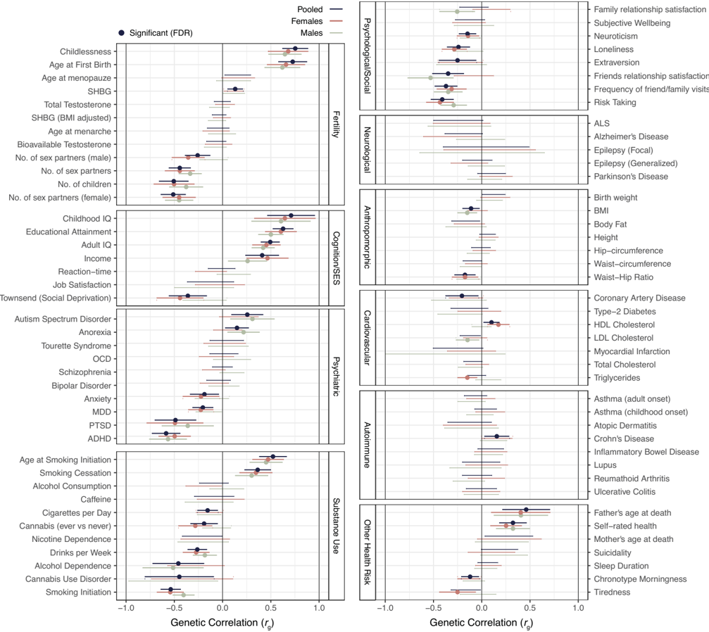
The headline 0.47 borrows directly from completed childlessness. A second route is to weight each adjacent phenotype's twin h² by its squared genetic correlation with sexlessness. r_g² is the proportion of additive-genetic variance shared between two traits: a phenotype that shares all its genes with sexlessness (r_g = 1) contributes its full heritability, one that shares none contributes nothing. Five adjacent phenotypes have both an LDSC r_g and a published twin h².

Phenotype	r_g (pooled)	r_g²	Twin h²	Weighted contribution
Completed childlessness	+0.75	0.57	0.47	0.264
Age at first birth	+0.73	0.53	0.30	0.159
Number of children (NEB)	−0.51	0.26	0.28	0.072
Number of sex partners	−0.44	0.20	0.24	0.047
Loneliness	−0.24	0.06	0.48	0.028

Table S1. r_g²-weighted triangulation of lifelong-sexlessness h² across five adjacent phenotypes for which both an LDSC genetic correlation and a published twin heritability exist; inputs are the same source values used in the main post's heritability and genetic-correlation tables.

Sum of weights 1.61, sum of weighted contributions 0.57. The weighted heritability is 0.35. This is a rough cross-check, not an estimator with formal guarantees: no correction is applied for assortative mating, non-additive variance, cohort drift, or uncertainty in the source estimates. It is useful because the inputs are published numbers and because it lands below, but near, the 0.47 completed-childlessness anchor.

Should the headline be uplifted?

The completed-childlessness data validate the calculation. In Verweij et al.'s (Verweij et al., 2017) Swedish twin data, male childlessness has MZ tetrachoric correlation 0.50 and DZ correlation 0.17; observed male MZ casewise concordance is 36.6%. At male prevalence 13.6% and h² = 0.46, Falconer's liability model predicts 34.5%. Plugging in the observed MZ liability correlation directly (0.50) predicts 36.9%. The model is calibrated for the proxy phenotype.

Autism shows the opposite lesson. For neurodevelopmental phenotypes, additive h² alone badly underpredicts observed concordance. Hallmayer et al. (Hallmayer et al., 2011): "Susceptibility to ASD has moderate genetic heritability and a substantial shared twin environmental component."

Observed values first:

Phenotype / source	Prevalence	Observed MZ concordance	h²/A used
Completed childlessness, F (Verweij et al., 2017)	12.0%	32.8% casewise	0.47
Completed childlessness, M (Verweij et al., 2017)	13.6%	36.6% casewise	0.46
Narrow autism (Bailey et al., 1995)	0.0175–0.10%	73% probandwise	0.91–0.93
Broad ASD (Tick et al., 2016; Ronald & Hoekstra, 2011)	5%	88% probandwise	0.93
Strict autism (Hallmayer et al., 2011)	0.5%	58% probandwise (M)	A = 0.37
Broad ASD (Hallmayer et al., 2011)	1.0%	77% probandwise (M)	A = 0.38

Table S2a. Liability-threshold validation — observed inputs: prevalence, observed MZ concordance, and the additive heritability used in the prediction.

And the model's predictions for those same rows:

Phenotype / source	Estimated from h²/A	Difference	Estimate from MZ r or A + C	Read
Completed childlessness, F (Verweij et al., 2017)	33.2%	+0.4 pp	same	Model matches.
Completed childlessness, M (Verweij et al., 2017)	34.5%	−2.1 pp	36.9% from MZ r = 0.50	Small upward miss.
Narrow autism (Bailey et al., 1995)	~46.7%	~−26 pp	~72.3% from MZ r = 0.978–0.983	h² alone underestimates.
Broad ASD (Tick et al., 2016; Ronald & Hoekstra, 2011)	69.5%	−18.5 pp	83.6% from MZ r = 0.98	Moderate underestimate.
Strict autism (Hallmayer et al., 2011)	5.4%	−52.6 pp	55.6% from A + C = 0.92	A alone is not the driver.
Broad ASD (Hallmayer et al., 2011)	8.0%	−69.0 pp	70.4% from A + C = 0.96	Same: A + C drives concordance.

Table S2b. Liability-threshold validation — predictions: predicted MZ concordance from h²/A alone, the gap to observed (Table S2a), and the prediction from the full MZ liability correlation (or A + C).

The autism rows recover observed concordance from total MZ liability correlation, not from additive h². That is an argument for using MZ r where you have it, not for replacing childlessness with autism. The proxy-choice argument committed us to childlessness, and childlessness calibrates.

Some modelling choices could push upward. Polderman et al. (Polderman et al., 2015) find that published h² tends to run below Falconer h² computed directly from twin correlations, partly because of ACE-vs-ADE model selection. Keller et al. (Keller et al., 2005) show that broad-sense H² can exceed narrow-sense estimates for personality dimensions, and Kendler et al. (Kendler et al., 1993) show that measurement error inflates E. These are general cautions, not sexlessness-specific corrections.

Downward pressure too. Border et al. (Border et al., 2022) show cross-trait assortative mating inflates published genetic correlations, which feeds back into the proxy strategy. The phenotype mixes voluntary religious abstinence, asexuality, situational isolation, illness, and involuntary non-partnering.

Net: 20.2% as the main age-30 male estimate, 28.5% as the generous h² = 0.60 upper-bound. The evidence does not justify an autism-style uplift.

Computing the concordance

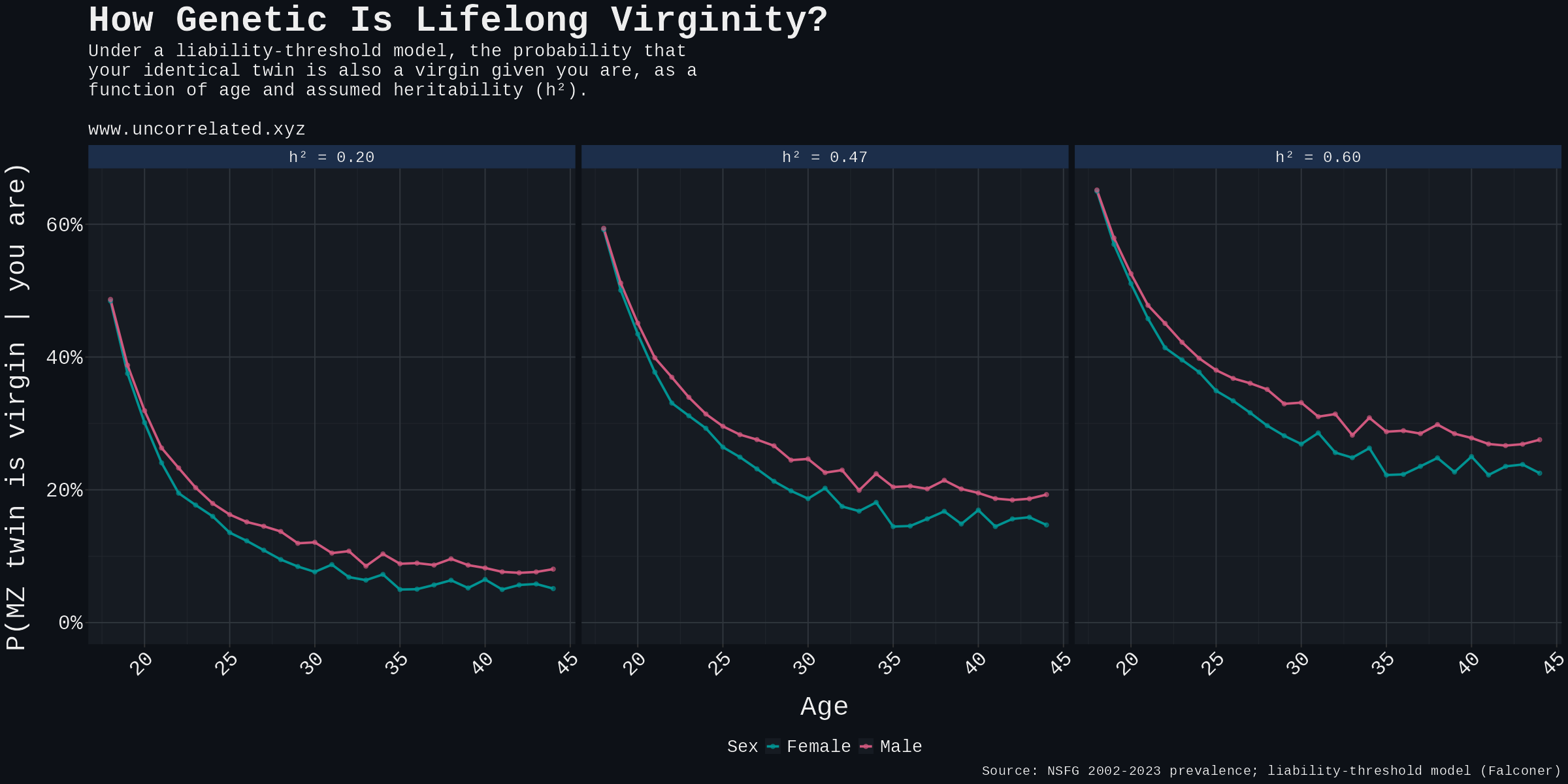
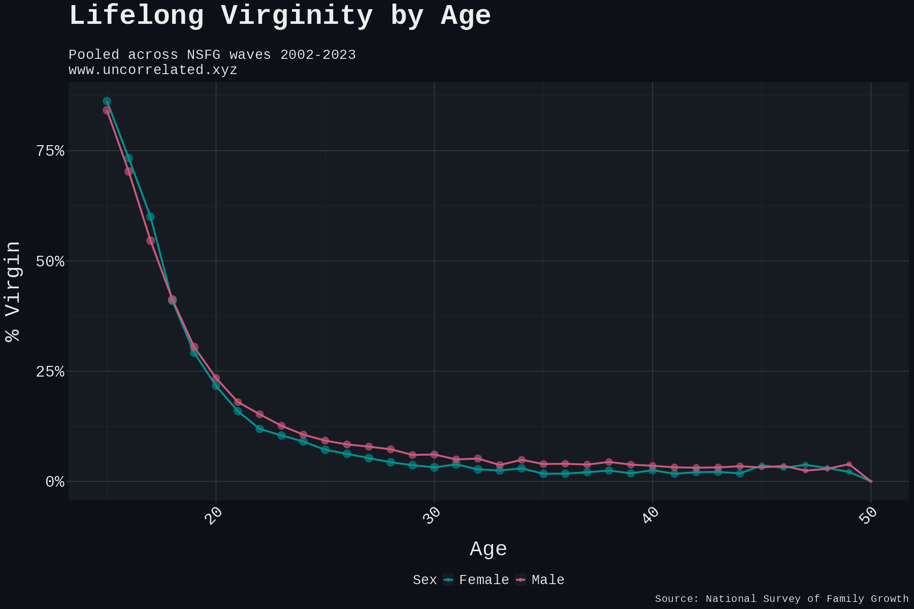
Method, four lines. (a) Take the pooled NSFG age-and-sex prevalence P. (b) Set T = Φ⁻¹(1 − P). (c) Compute the bivariate-normal upper-right tail P(L₁ > T, L₂ > T) at correlation h². (d) Divide by P for the conditional concordance. Analytic via R's mvtnorm::pmvnorm and Monte Carlo with 10⁶ twin pairs agree to three decimal places.

Age	F prevalence	M prevalence	Twin concordance, F	M
20	14.5%	22.1%	22.5%	30.6%
25	4.4%	8.2%	9.6%	14.9%
30	1.7%	3.8%	5.0%	8.7%
40	1.1%	0.9%	3.7%	3.0%

Table S3. Sensitivity at h² = 0.20 (low anchor).

Age	F prevalence	M prevalence	Twin concordance, F	M
20	14.5%	22.1%	44.3%	51.4%
25	4.4%	8.2%	29.8%	36.5%
30	1.7%	3.8%	22.3%	28.5%
40	1.1%	0.9%	19.4%	17.9%

Table S4. Sensitivity at h² = 0.60 (generous upper bound).

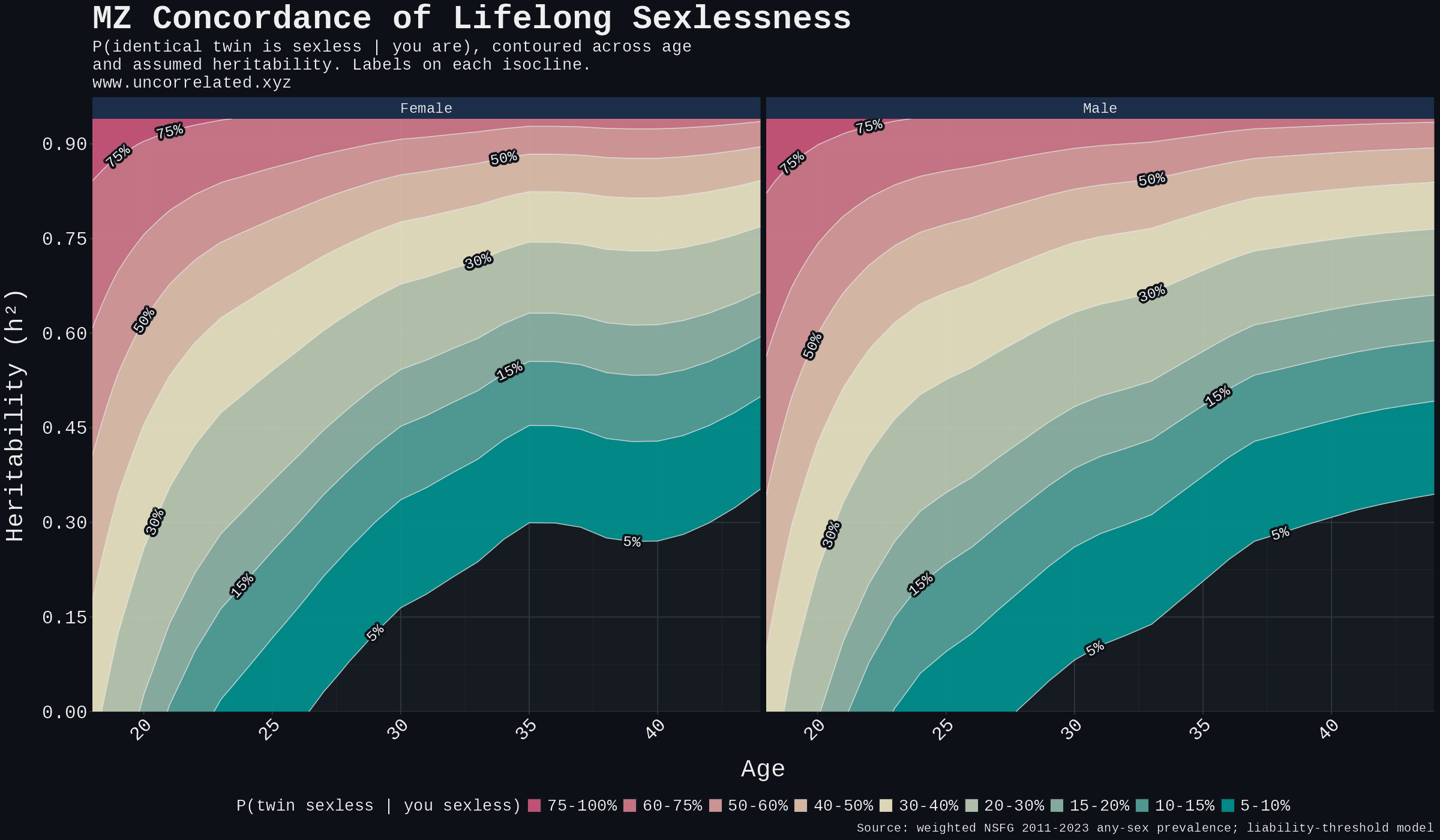Figure S1. Predicted MZ-twin concordance contoured over the full (age, h²) plane.

Autism and rare variants: the Bayes share

A back-of-the-envelope estimate of autism's share of the male sexless tail at 30:

P(autism | sexless at 30) = P(sexless | autism) × P(autism) / P(sexless) ≈ 0.50 × 0.01 / 0.038 ≈ 13%.

Using P(sexless | autism) ≈ 0.50, autism prevalence ~1%, and male age-30 sexlessness prevalence ~3.8%. The calculation is deliberately crude: it says autism could plausibly account for a noticeable minority of the male sexless tail, not that autism is the main axis of the phenotype. Even if the 0.50 input is moved around substantially, the conclusion remains the same: autism is a pathway into sexlessness, but it is too uncommon to explain most of it.

How s_het burden is calculated

Gardner et al. (Gardner et al., 2022) calculate a separate burden score for each individual i and variant class v:

$$\text{burden}_{i,v} = 1 - \prod_{g \in G_{i,v}} \left(1 - s_{\text{het},g}\right)$$

where:

• $G_{i,v}$ is the set of genes in which individual i carries at least one private, heterozygous variant of class v.
• $s_{\text{het},g}$ is the per-gene selection coefficient from Weghorn et al. (Weghorn et al., 2019), with Cassa et al. (Cassa et al., 2017) used as a robustness check. Gardner's main Weghorn scores cover 16,189 protein-coding genes.

The formula is the same for genic deletions, PTVs, missense variants, synonymous variants, and duplications. What changes is the qualifying gene set. In the post, only deletions and PTVs matter because those are the strong Gardner channels used for the sexlessness calculation.

Gardner's "meta" estimate is not a combined per-individual burden. It is a fixed-effects meta-analysis of the deletion-burden and PTV-burden regression coefficients. Gardner does not publish a deletion+PTV joint distribution, and the paper does not report a statistic such as "combined burden ≥ 0.15." A true per-individual union score would require the individual-level deletion/PTV overlap.

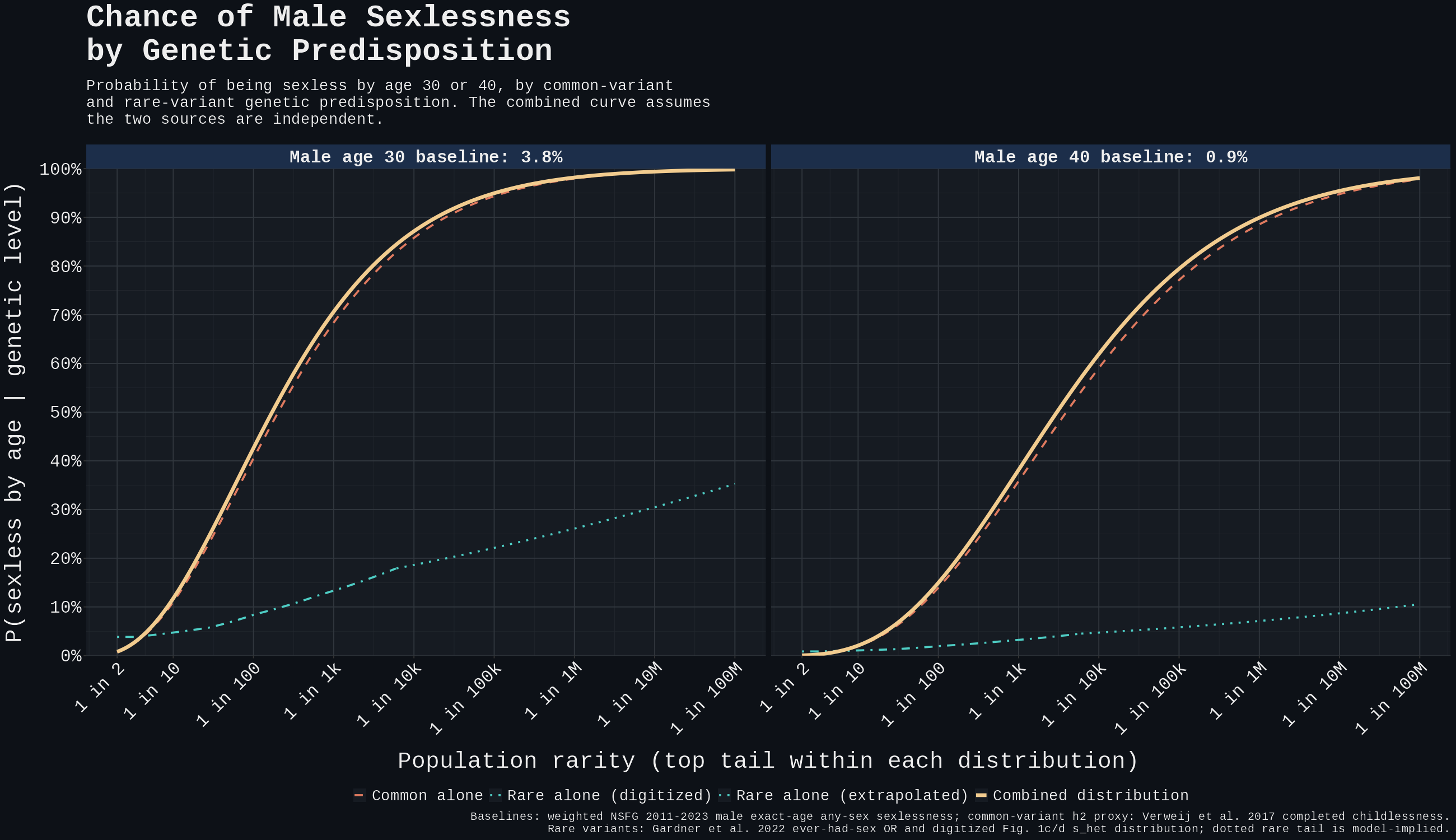
For the rare-vs-common plot, I therefore use an effective rare-burden distribution: digitise Gardner Fig. 1c/d, then weight the deletion and PTV histograms by the inverse-variance weights from Gardner's male ever-had-sex meta-analysis (Supplementary Table 4, Fig. 2b). Those weights are 24.5% deletion and 75.5% PTV. This matches the Gardner OR used in the plot (male ever-had-sex OR = 0.059 per unit of $s_{\text{het}}$ burden), but it should be read as a plotting approximation, not a burden Gardner directly observed.

Digitisation details: render the Gardner PDF, detect the log y-axis ticks, extract the male and female bar tops in Fig. 1c/d, average the sexes, and anchor-adjust the tails to Gardner's exact reported $s_{\text{het}} \geq 0.15$ proportions: 0.56% and 0.55% for deletions; 4.60% and 4.59% for PTVs.

Bin	Deletion %	PTV %	Effective rare %
0	96.40	61.81	70.28
(0, 0.15]	3.05	33.59	26.11
(0.15, 0.30]	0.383	3.410	2.669
(0.30, 0.45]	0.113	1.007	0.788
(0.45, 0.60]	0.0349	0.164	0.132
>0.60	0.0235	0.0146	0.0168

The effective upper tail is therefore about 3.61% above $s_{\text{het}} = 0.15$, 0.94% above 0.30, 0.15% above 0.45, and 0.017% above 0.60. Log-linear interpolation inside bins gives approximate percentiles of $s_{\text{het}} \approx 0.13$ at the 95th percentile, 0.29 at the 99th, and 0.48 at the 99.9th.

The combined rare + common plot then treats this effective rare-burden distribution as independent of common-variant liability and combines the two effects on the odds scale. That independence assumption is ours; Gardner supplies the rare-variant slope and the two single-channel burden histograms, not a combined rare+common model.