Unravelling Cold Winters Theory with Ancient Genomes

Table of Contents

TL;DR

• We tested cold winters theory using polygenic scores from ancient genomes matched to historical winter temperatures dating back 21,000 years.

• Height and educational attainment polygenic scores significantly correlate with colder winters (p < 0.001), even after controlling for ancestry, in both modern and ancient samples.

• Cognitive ability and non-cognitive ability polygenic scores show no significant correlation with winter temperatures after ancestry controls.

• Cold winters theory receives partial support. The correlations exist but are weaker than proponents might expect.

---

A few weeks ago I was chatting with Davide Piffer, and we arrived at the topic of ancient genomes and cold winters.

Cold winters, proposed by Richard Lynn, is an old theory that individuals subjected to hard cold winters were evolutionarily selected for long-term planning and intelligence; those who didn’t prepare died. It’s easy to imagine how adaptation for these traits would then give rise to agriculture or future advancements along the human evolution and tech tree to the civilization we have today.

Piffer told me that, controlling for ancestry, there was no correlation between latitude and an ancient genome’s polygenic score for cognitive ability. Height polygenic scores survived the controls, which made sense: taller, larger bodies have smaller surface areas relative to their volume, preserving heat. This is a classic ecogeographic pattern (Bergmann’s rule). But the cognitive measures didn’t show the same robustness.

Not long after, he published a substack article on the topic. I then tweeted his results, which went viral relative to my previous posts.

Summary of Piffer’s Post

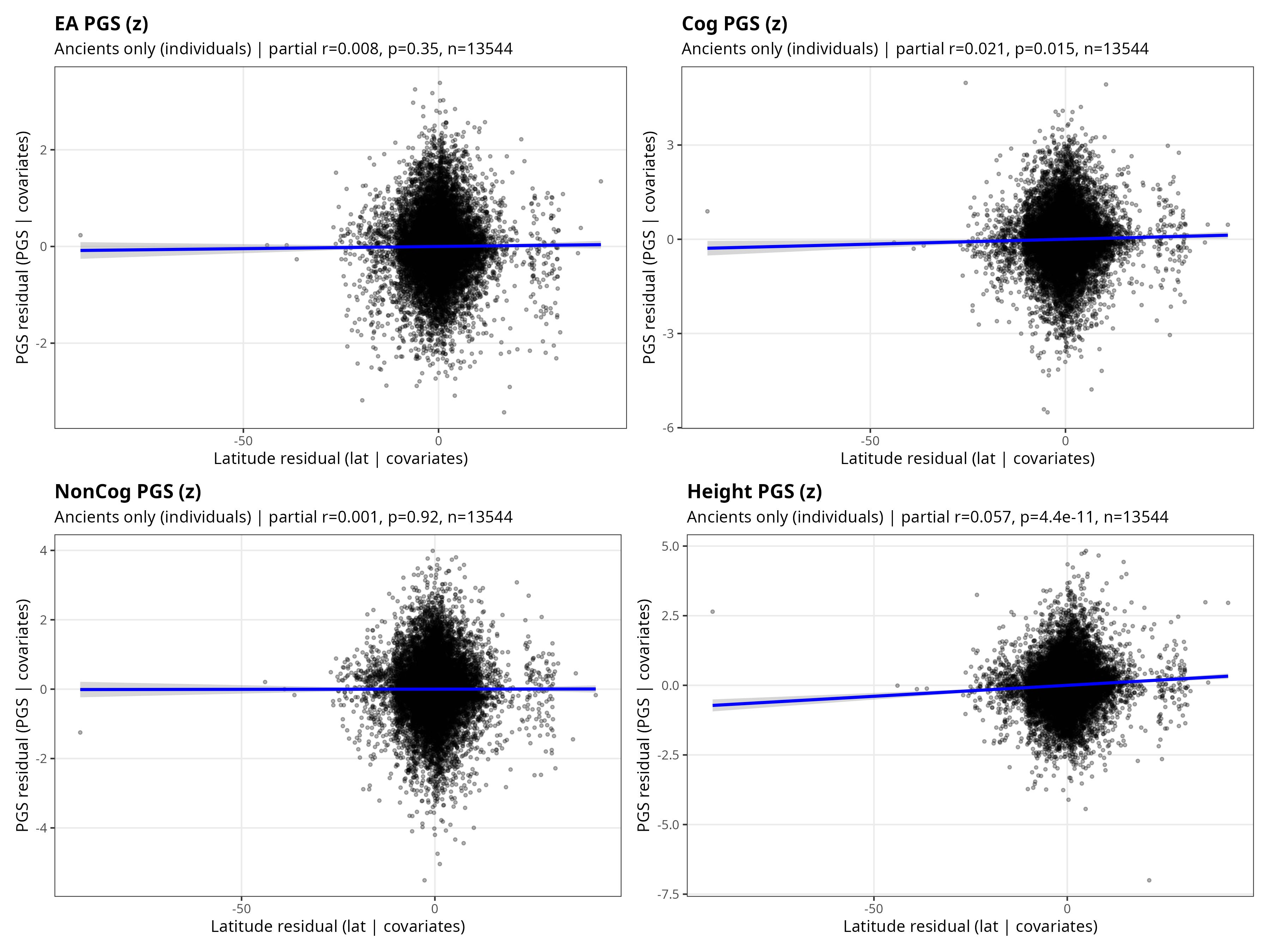
Piffer used polygenic scores for educational attainment (EA), cognitive ability (Cog), non-cognitive ability (NonCog), and height, tested against absolute latitude as a proxy for climate. He controlled for the first 10 genome-wide principal components (ancestry), genomic coverage (data quality), and time (years before present). He ran analyses on ancient samples, modern samples, and pooled data, at both individual and group levels.

His findings: in naive models without ancestry controls, all traits showed strong latitude gradients. After PC adjustment, EA, Cog, and NonCog lost their latitude signal. Height alone retained a significant positive association with latitude across all samples (partial r = 0.05-0.06, p < 10^-10).

Piffer was explicit about the limitations of his approach. He acknowledged that PC adjustment is inherently conservative: it asks whether there’s a latitude effect that survives conditioning on genome-wide ancestry. If climate shaped ancestry distributions over deep time rather than exerting parallel selection within ancestries, PCs would absorb much of that signal by design. He framed his results as “evidence against a strong, ancestry-independent, global latitude gradient, not as a claim that climate played no role at all.”

He concluded by calling for more direct tests: “Latitude is a blunt proxy, and the theory’s core prediction concerns winter severity and seasonality over many generations, not latitude per se. More direct tests would require explicit measures of winter climate, seasonal volatility, and within-continent comparisons where environmental gradients can be evaluated without being dominated by deep ancestral structure.”

---

This article is that test. Piffer and I teamed up to run a more direct analysis, using actual winter temperatures rather than latitude, and applying a different set of controls and methods. Working together let us move faster than we would have separately. We shared datasets old and new, retested methods more systematically, and bounced ideas off each other. This post and his substack article are the result.

From Latitude to 21,000 Years of Winter

I needed historical temperature data going back far enough to match the ancient genomes. I found CHELSA-TRACE21k, a dataset of geospatial temperature estimates at century-level resolution dating back 21,000 years.¹ Below are daily minimum average temperatures for January in Europe, 10,000 before present.

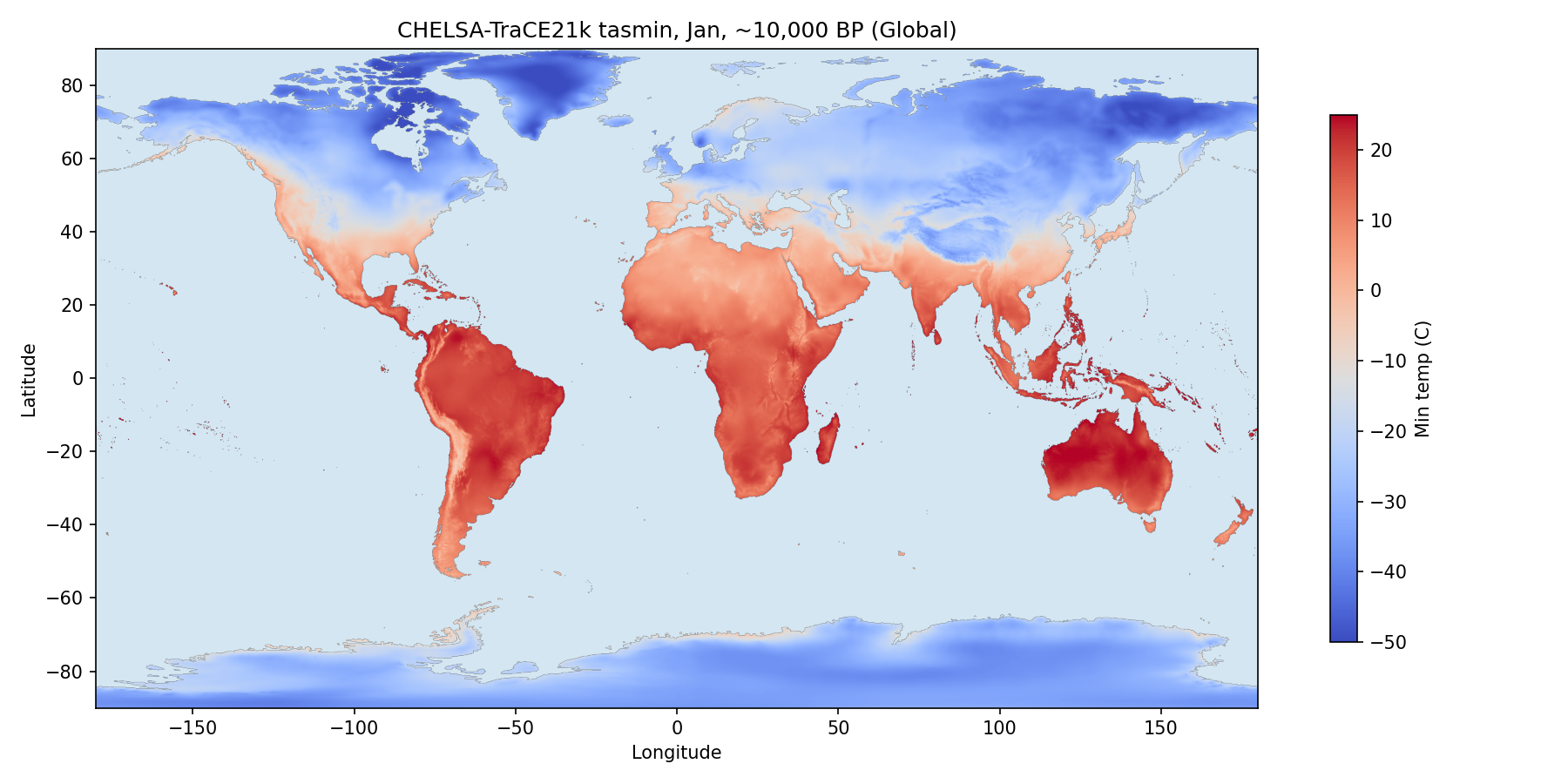
For each genome, we calculated winter temperature by averaging temperatures within a 25 km radius of its location, excluding bodies of water. We used January for Northern Hemisphere samples and July for Southern Hemisphere samples, then matched each genome to the nearest century in the temperature data (a sample 8,475 years before present uses data from 8,500 years before present).²

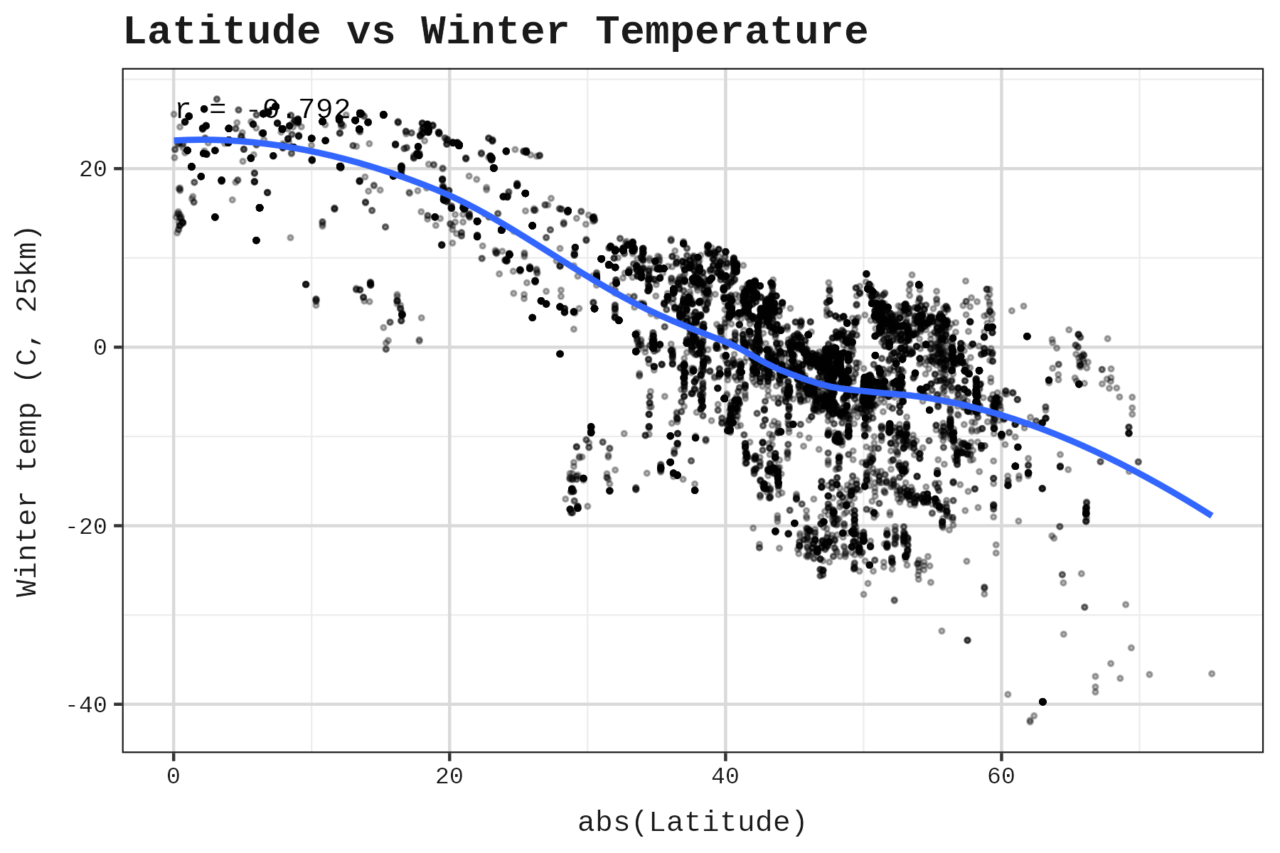
The correlation between absolute latitude and winter temperature was r = -0.792. Strong, but not perfect. If latitude were a perfect proxy for winter severity, switching to actual temperatures wouldn’t matter. The imperfect correlation means there’s information in the temperature data that latitude alone doesn’t capture.

A multicollinearity check confirms all three climate variables can be used in the same model (VIF = 1 / (1 - r²), where r² is from regressing each predictor on the others):

Predictor	Against	r	VIF
Winter	Summer + Latitude	0.797	2.74
Summer	Winter + Latitude	0.460	1.27
Latitude	Winter + Summer	0.799	2.77

All VIFs below 5, so multicollinearity is acceptable.

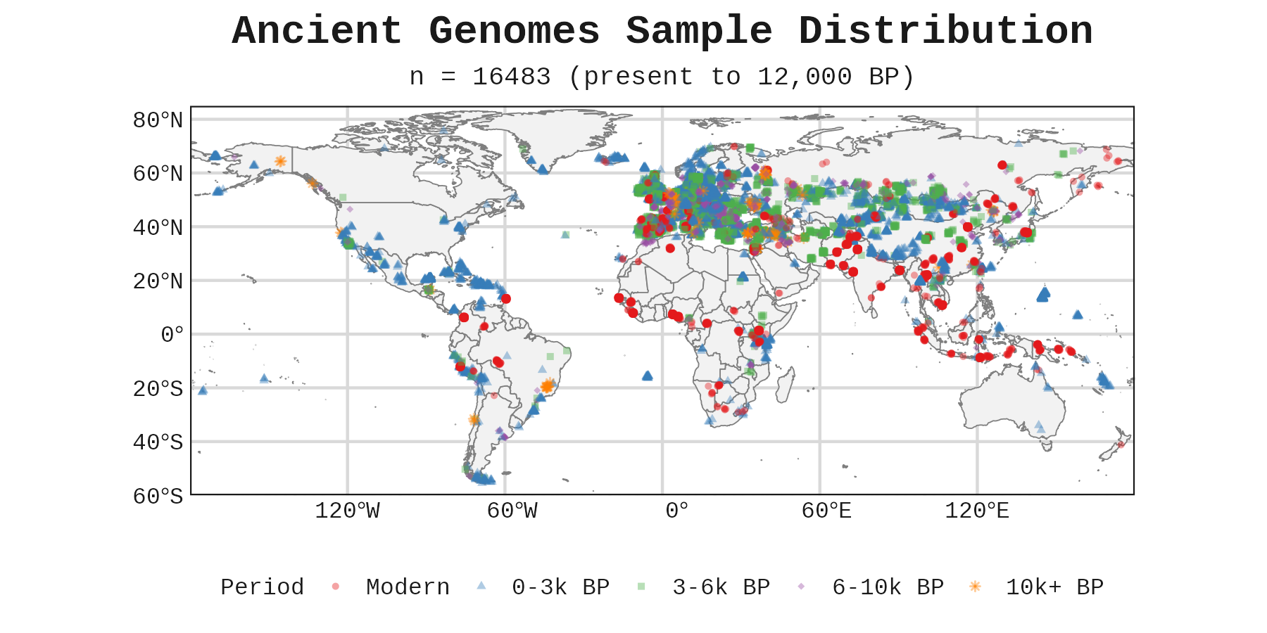
The ancient genomes come from an amalgamation of sources. Piffer provided the data along with four polygenic scores (EA, height, cognitive ability, and non-cognitive ability), principal components up to PC20, and latitude/longitude coordinates for each sample.

Controlling for Ancestry

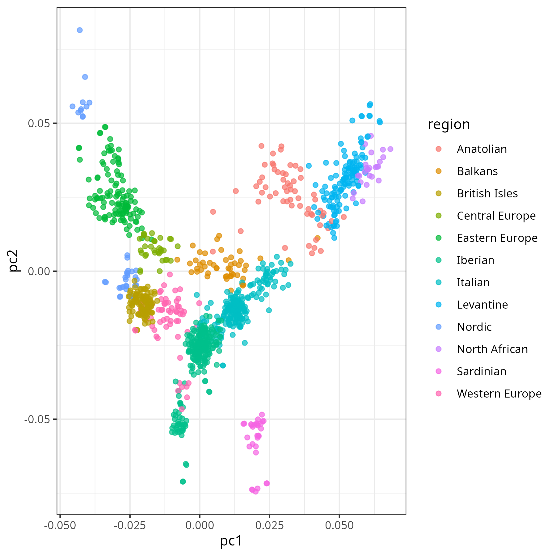
The previous analysis controlled for ancestry using principal components (PCs). The first PC is the variable that explains the most variation in the genomes, the second explains the second most, and so on. The first two PCs are often plotted to visualize population structure. Since PCs are mutually uncorrelated by definition, they provide a clean “map” of ancestry. Here’s Europe:

Controlling for too many PCs risks absorbing not just ancestry, but the very trait variation we’re trying to detect. At that point, any correlation would be rendered non-significant by construction. Additionally, more controls crowd out the regression: each added variable, even if meaningless, increases noise in the other estimates.

So, the question is: what’s the minimum number of PCs that adequately controls for ancestry?

We ran two tests to find this minimum.

First, at what point do additional PCs face diminishing returns for predicting polygenic scores? If additional PCs continue to improve prediction accuracy, ancestry retains explanatory power. Once predictions plateau, we’ve captured the ancestry component, and further PCs risk absorbing trait variance.

Second, at what point do additional PCs face diminishing returns for predicting a genome’s latitude and longitude? Latitude is our proxy for cold winters, so this tells us when geographic ancestry has been adequately controlled. Beyond that point, additional PCs no longer capture geographic structure.

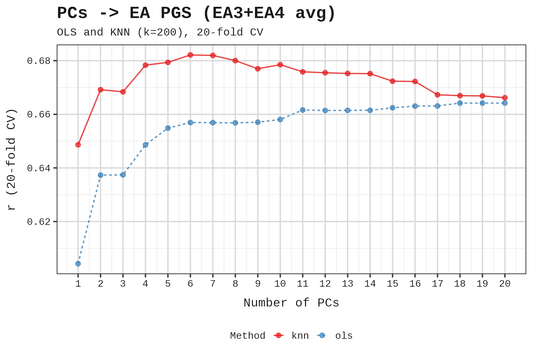
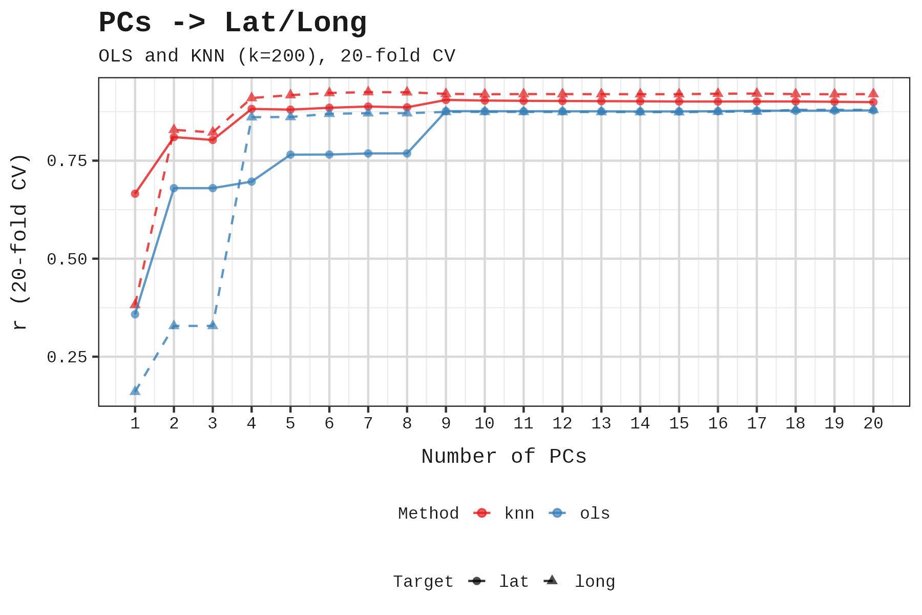
Both tests point to the same answer: 3 to 6 PCs. The correct number likely lies at the intersection of these two constraints: enough to capture geographic ancestry, but before we start absorbing trait variance. We settled on 6 to be generous.

Results

We controlled for ancestry (6 PCs) and date using piecewise regression, since the relationship between years before present and EA is non-linear.

To check robustness, we tested how results changed as we added more PCs. EA and height maintained significance up to PC9.

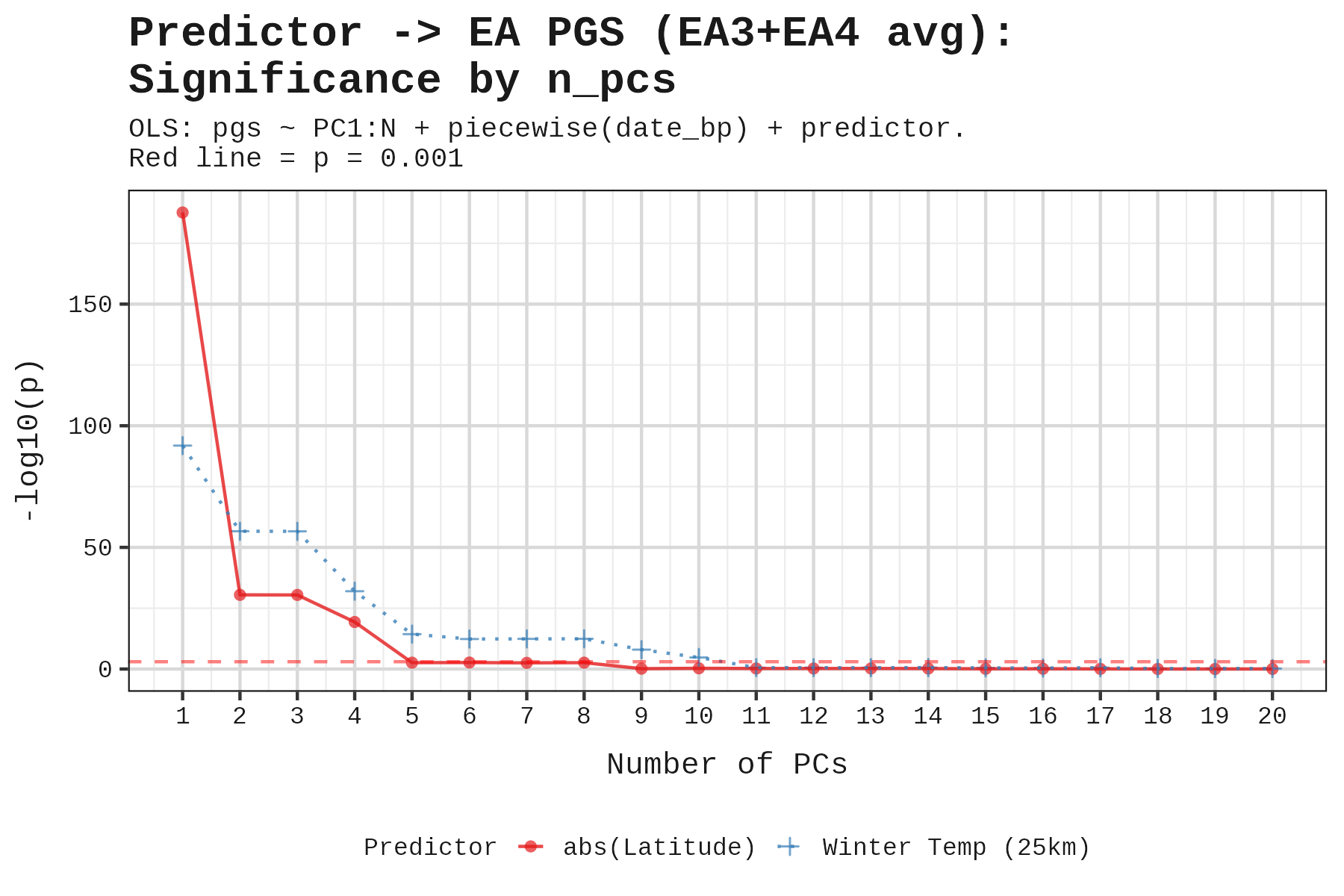
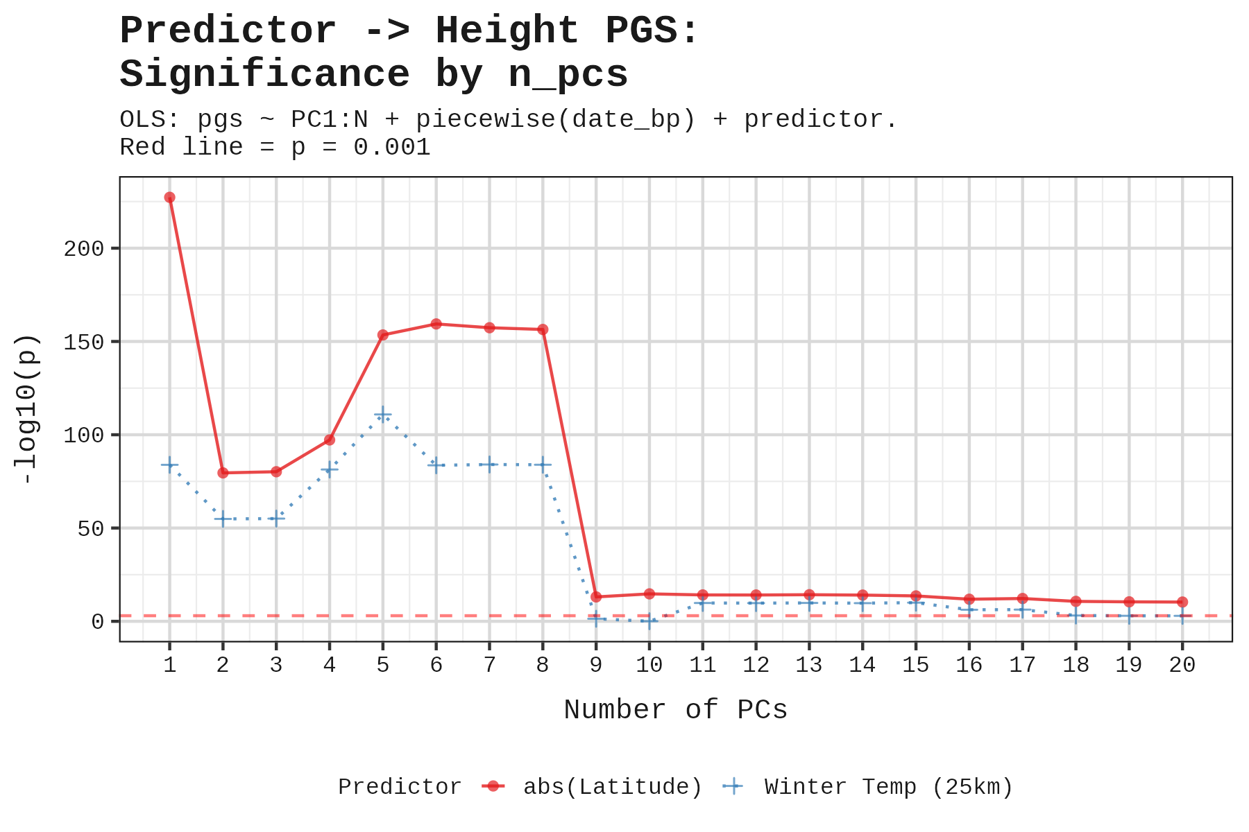
Using 6 PCs, here are the results:

Trait	Predictor	Beta	p
Educational Attainment	Latitude	0.00195	0.002
Educational Attainment	Winter Temperature	-0.00467	4.7e-13
Height	Latitude	0.0209	4.0e-160
Height	Winter Temperature	-0.0154	2.4e-84
Cognitive Ability	Latitude	0.00020	0.81
Cognitive Ability	Winter Temperature	-0.00041	0.62
Non-Cognitive Ability	Latitude	-0.00013	0.87
Non-Cognitive Ability	Winter Temperature	-0.00076	0.35

Height and educational attainment show significant effects; cognitive and non-cognitive ability do not.

The betas are in standard deviation units per degree. To put this in perspective, consider a 30°C shift (roughly the difference between Mediterranean and Scandinavian winters). For height, a 30°C decrease in winter temperature is associated with a 0.46 SD increase in height PGS. For educational attainment, a 30°C decrease is associated with a 0.14 SD increase. The winter betas are negative because colder temperatures (lower values) predict higher polygenic scores.

We also ran a regression with winter temperature, summer temperature, and latitude together. As discussed earlier, multicollinearity between these variables is low (VIF < 3), so the betas remain stable. When correlated predictors compete in the same model, the one capturing the true causal signal typically retains or increases its effect size, while redundant predictors attenuate.

Trait	Predictor	Beta	p
Educational Attainment	Winter Temperature	-0.00808	1.80e-15
Educational Attainment	Summer Temperature	+0.00439	4.02e-03
Educational Attainment	Latitude	-0.00305	1.52e-03
Height	Winter Temperature	+0.00260	0.033
Height	Summer Temperature	-0.00804	1.22e-05
Height	Latitude	+0.02107	4.85e-73

For EA, colder winters and warmer summers independently predict higher polygenic scores. For height, latitude dominates: higher latitudes predict taller stature, with cooler summers contributing independently.

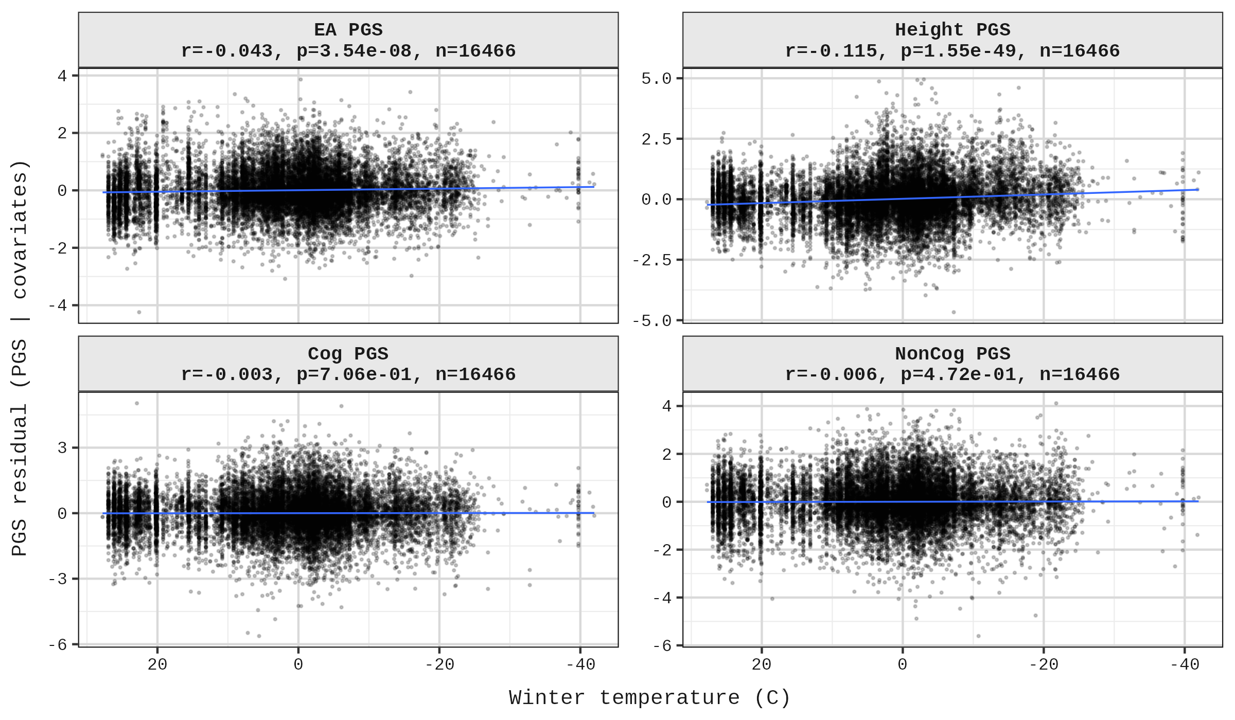
The table results come from a regression predicting each trait from the climate variable, controlling for ancestry (6 PCs) and date. To visualize these relationships, we removed the effect of the controls from the trait, then plotted what remains against each predictor. This isolates the predictor’s effect but may look slightly different from the table betas, which estimate all predictors simultaneously.

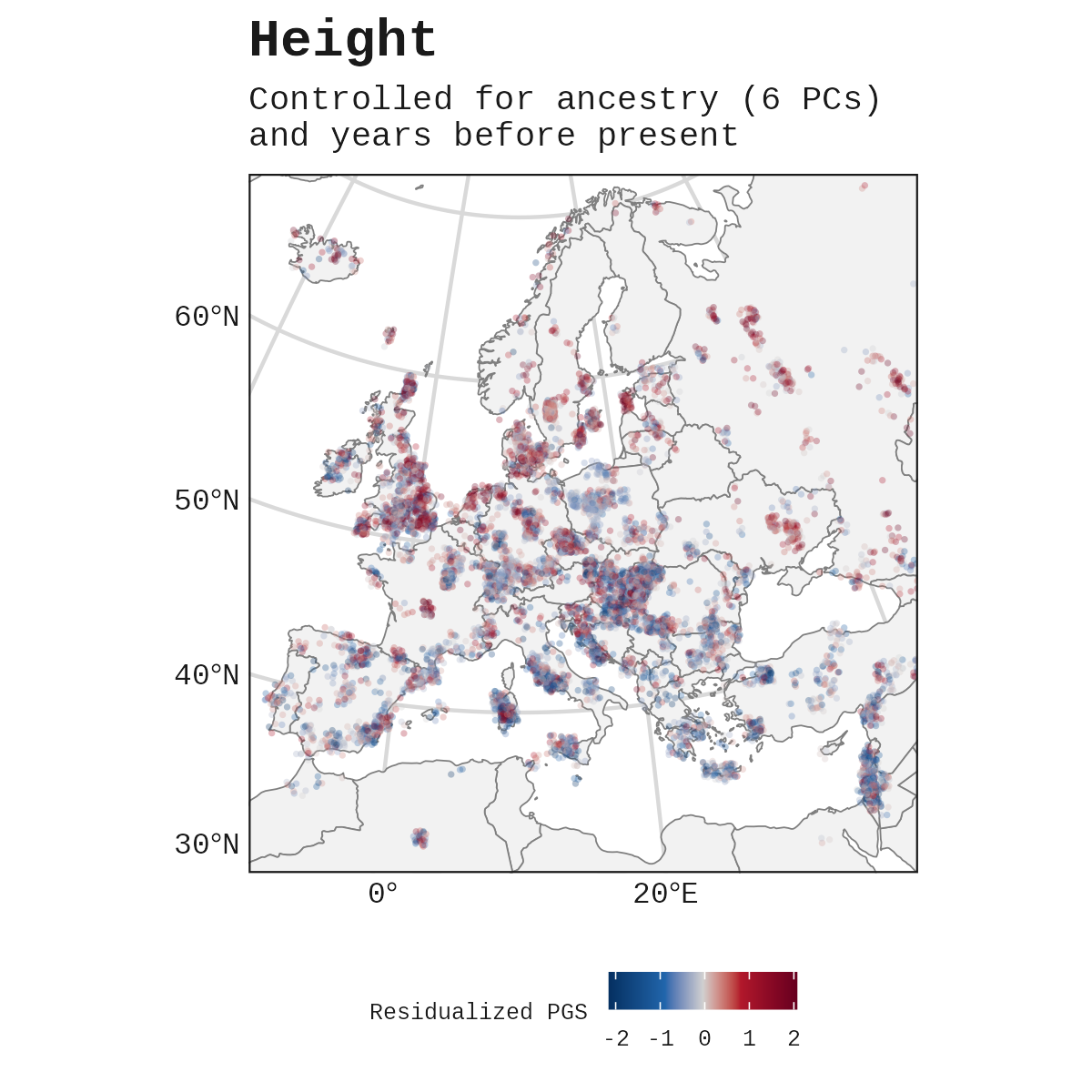
A different way to visualize this: plotting the controlled height PGS onto a map of Europe. This is after removing the effect of ancestry and date.

The dataset also includes 3,111 modern samples (date BP = 0). Running the same regression on moderns corroborates the main findings: for EA, winter temperature remains the dominant predictor, while summer and latitude lose significance. For height, all three predictors remain significant, with latitude showing the strongest effect.

But These Correlations are Tiny!

They are small, but multiple factors suppress them.

First, linkage disequilibrium. Polygenic scores trained on one ancestry group become less accurate when applied to others, not biased in any direction, just noisier. The ancient samples span the globe and date back tens of thousands of years, which increases measurement error and attenuates correlations.

Second, polygenic scores aren’t that predictive to begin with. The height PGS accounts for 40-45% of phenotypic variance in European ancestry populations. The EA PGS (EA3, EA4) accounts for only 12-16%. Since height’s polygenic score captures far more of the trait’s variance, we’d expect stronger and more detectable effects for height, which is exactly what we observe.

Despite all this, the correlations survived and remained statistically significant.

Is cold winters theory dead? I don’t think the answer is a simple yes or no. The correlations aren’t what proponents might have expected, but they’re not zero either. Detractors can’t claim the theory is meaningless.

Appendix

Results on modern samples only:

Model	Predictor	Beta	p
Full	Winter	-0.01034	9.31e-05
Full	Summer	-0.00071	0.85 (NS)
Full	Latitude	-0.00114	0.62 (NS)
Winter only	Winter	-0.00952	6.69e-12
Latitude only	Latitude	+0.00680	3.07e-07

Model	Predictor	Beta	p
Full	Winter	+0.01393	8.49e-06
Full	Summer	-0.03391	7.12e-14
Full	Latitude	+0.02294	4.29e-17
Winter only	Winter	-0.01181	1.39e-12
Latitude only	Latitude	+0.01513	1.57e-21