Supplementary Materials

Downloads

Appendix

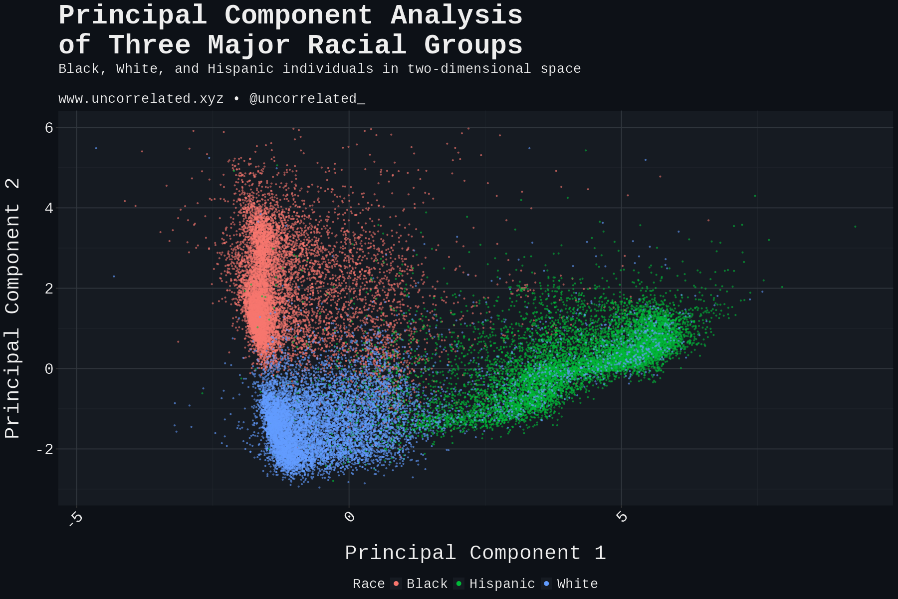
Mathematical Formulation of Bias for Simulation

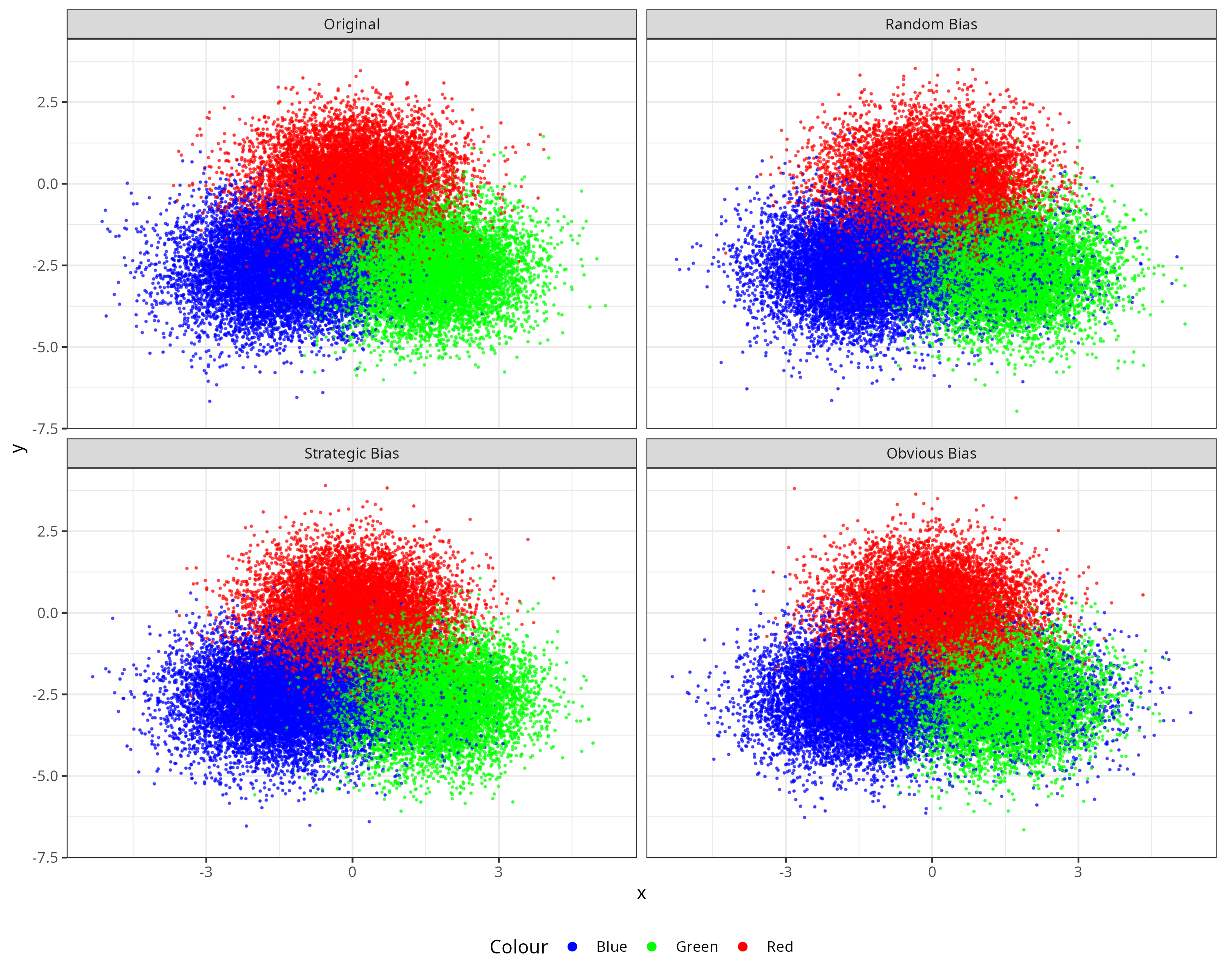
For each bias scenario, we systematically reassigned 10% of Greens to Blue classification, with the selection mechanism varying according to the specific bias type being simulated.

Let the Blue centroid be represented by coordinates $(c_x, c_y)$ in our two-dimensional feature space. For each Green point $g_i$ with coordinates $(x_i, y_i)$, we calculated the Euclidean distance to the Blue centroid:

$$d_i = \sqrt{(x_i - c_x)^2 + (y_i - c_y)^2}$$

The bias assignment probabilities were then defined using exponential functions that create distinct selection patterns for Strategic and Obvious bias types:

$$P_{\text{strategic}}(i) = \exp(-d_i)$$ $$P_{\text{obvious}}(i) = \exp(d_i)$$

These formulations ensure that Strategic bias preferentially selects Green individuals closest to the Blue centroid (higher probability for smaller distances), while Obvious bias preferentially selects those most distant from the Blue centroid (higher probability for larger distances).

We then used weighted sampling on these probabilities (higher values more likely to be sampled) for each respective scenario to produce our end-product simulated datasets:

• Strategic bias: weights proportional to $P_{\text{strategic}}(i) = \exp(-d_i)$
• Obvious bias: weights proportional to $P_{\text{obvious}}(i) = \exp(d_i)$
• Random bias: uniform weights (weights = 1 for all individuals)

Model Training and Evaluation on Simulations

Following bias introduction, we trained multinomial logistic regression models on each simulated dataset using the simple formula race ~ x + y, where x and y represent the two-dimensional coordinates. This straightforward approach mirrors our linear modeling strategy for the real-world data while maintaining interpretive clarity.

To address class imbalances created by the reassignment process, we implemented inverse frequency weighting:

$$w_j = \frac{N_{\text{total}}}{3 \times N_j}$$

where $w_j$ represents the weight for class $j$, $N_{\text{total}}$ is the total sample size, and $N_j$ is the number of observations in class $j$ after bias introduction. This weighting scheme ensures that our models optimize for balanced performance across all three groups. This was done to correct for the imbalance produced by reassignment, and for consistency with the method used on the real dataset.

The simulation process generates four distinct datasets: the original unbiased dataset plus three variants incorporating Random, Strategic, and Obvious bias patterns, respectively. These four scenarios are visualized, illustrating how each bias type creates characteristic distortions in the group assignment patterns.